ABSTRACT
Supra-arcade fans are highly dynamic structures that form in the region above post-reconnection flare arcades. In these features the plasma density and temperature evolve on the scale of a few seconds, despite the much slower dynamics of the underlying arcade. Further, the motion of supra-arcade plasma plumes appears to be inconsistent with the low-beta conditions that are often assumed to exist in the solar corona. In order to understand the nature of these highly debated structures, it is, therefore, important to investigate the interplay of the magnetic field with the plasma. Here we present a technique for inferring the underlying magnetohydrodynamic processes that might lead to the types of motions seen in supra-arcade structures. Taking as a case study the 2011 October 22 event, we begin with extreme-ultraviolet observations and develop a time-dependent velocity field that is consistent with both continuity and local correlation tracking. We then assimilate this velocity field into a simplified magnetohydrodynamic simulation, which deals simultaneously with regions of high and low signal-to-noise ratio, thereby allowing the magnetic field to evolve self-consistently with the fluid. Ultimately, we extract the missing contributions from the momentum equation in order to estimate the relative strength of the various forcing terms. In this way we are able to make estimates of the plasma beta, as well as predict the spectral character and total power of Alfvén waves radiated from the supra-arcade region.
1. INTRODUCTION
Supra-arcade fan structures have been observed since the beginning of X-ray and EUV imaging of the solar corona. Often referred to as current sheets, these are typically found above the dominant polarity inversion line of solar active regions and are anchored at the apex of an arcade of newly formed flare loops. The fan is, therefore, spatially coincident with the assumed current sheet that defines a rotational discontinuity in the open magnetic field above the arcade. We are careful, however, to distinguish the emissive structure, referred to as a Current Sheet/Thermal Halo (CSTH) by McKenzie (2013), from the actual supra-arcade current sheet, which may be significantly thinner (Seaton & Forbes 2009) and need not, necessarily, contribute significantly to the supra-arcade emission.
The energy balance in the supra-arcade region has been a topic of interest since the first observations of Supra-Arcade Downflows (SADs) by McKenzie & Hudson (1999). Previously, many authors had suggested that the magnetically dominated forcing typified in active region cores held true for supra-arcade structures as well. However, the dynamics of SADs show evidence of Rayleigh–Taylor-type instabilities (Guo et al. 2014), while the oscillations along the edges of supra-arcade density lanes that were considered by Verwichte et al. (2005) may be indicative of Kelvin–Helmholtz wave excitation, both of which suggest a nontrivial contribution from the plasma pressure. Indeed, McKenzie (2013) estimated that the plasma β, which is the ratio of thermal to magnetic energy densities, should be of order unity or greater in the 2011 October 22 event, with significant variation within the structure itself.
It is the aim of this paper to improve our understanding of the dynamics exhibited by supra-arcade fan structures. As a case study, we considered the supra-arcade structure that formed on the northwest (NW) limb on 2011 October 22—the same event considered by Savage et al. (2012), McKenzie (2013), and Hanneman & Reeves (2014). Owing to the predominantly north–south alignment of the polarity inversion line and its position on the limb, the line of sight is taken to be normal to the plasma sheet. This vantage point allows us to estimate the plasma motion and magnetic evolution in the plane of the sky.
The organization of this paper is as follows. In Section 2 we describe our methods for estimating the plasma density and the associated velocity field. Section 3 describes our method for inferring the evolution of the supra-arcade magnetic field. Then, in Section 4 we compare the dynamics of the fluid and the magnetic field in order to estimate the radiated wave spectra, energy balance, and, ultimately, plasma pressure. Our results are summarized in Section 5.
2. OBSERVED PLASMA EVOLUTION
The 2011 October 22 event occurred on the NW limb and was observed by the Atmospheric Imaging Assembly (AIA) on board the Solar Dynamics Observatory (Lemen et al. 2012) at 12 s cadence and 0.6″ (435 km) per pixel resolution in each of the seven extreme-ultraviolet (EUV) channels ranging from 94 to 335 Å. We retrieved the data from all seven EUV passbands so that we might disambiguate the plasma motion from possible temperature effects. The data were retrieved using the vso_search and vso_get routines (Hill et al. 2009), which are available through SolarSoft (Freeland & Handy 1998). Each image was cropped using the read_sdo routine and then prepped and normalized via aia_prep. The resulting image cube contains a little over 3 hr of uninterrupted high-cadence, multispectral data.
For this event, we assumed that the supra-arcade fan, which exhibits strong emission in the 131 Å passband (Figure 1), consists of a halo of plasma surrounding a current sheet, which supports a 180° rotational discontinuity within an otherwise smooth, predominantly radial magnetic field. The column depth is assumed to be uniform and small compared to the length scale for variation of the magnetic field along the line of sight, and we are therefore able to treat the problem two-dimensionally, with the direction along the line of sight understood to be ignorable and the bulk velocity and magnetic fields lying purely in the plane of the sky.
Figure 1. Representative frame from the 2011 October 22 event on the NW limb. The event is shown with three different fields of view in the AIA 131 Å channel, which is dominated by Fe xxi at approximately 107 K.
(An animation of this figure is available.)
Download figure:
Video Standard image High-resolution image2.1. Differential Emission Measure Inversion
We begin our analysis with the differential emission measure (DEM), which we determined using the fast iterative regularized DEM inversion code developed and described by Plowman et al. (2013). Omitting the 304 Å channel (J. Plowman 2014, private communication), the inversion was performed with the six remaining channels for a reduced field of view (512 × 512 pixels) at full resolution, with a cadence of 12 s spanning from 11:35 UT to 15:00 UT.
Inspection of the spatially averaged DEM in the supra-arcade fan confirmed the results of Hanneman & Reeves (2014), in which the entire fan structure exhibits relatively stable emission below T ∼ 106.5 K and a highly dynamic contribution from plasma with temperatures of 106.5 K and above. We interpret this result to mean that the lower temperature contribution is due to a uniform, low-density, relatively cool plasma that extends significantly along the line of sight (i.e., the foreground and background corona), while the high-temperature contribution is the result of plasma that is confined to the supra-arcade plasma sheet, with a much higher density and a relatively short column depth.
Anticipating that the dynamics in the 131 Å channel would be associated with the supra-arcade plasma sheet, which we wanted to isolate from the rest of the diffuse corona, we considered only the high-temperature contribution to the DEM. In order to isolate this higher-density plasma, we multiplied the complete DEM, (T), by a high-temperature filter,

which increases smoothly from zero to one over an interval of about 1 MK, centered on log10T = 6.5. We then constructed the total filtered column emission measure, f, by integrating the filtered DEM across all temperatures:

This integrated emission is taken as the total emission measure associated with the supra-arcade region, with minimal contribution from the diffuse corona. Examples of the filtered and unfiltered DEM are depicted in Figure 2. Figure 3 depicts the total column emission measure with and without the high-temperature filter.
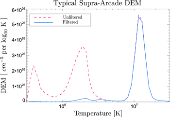
Figure 2. Representative example of the spatially averaged, filtered and unfiltered DEMs are depicted in solid blue and dashed red, respectively. This example is taken during the height of supra-arcade activity, at approximately 13:00 UT. Note the suppression of emission measure below  . The filtered DEM retains only the high-temperature plasma, which is assumed to be the primary contributor to the supra-arcade fan emission.
Download figure:
Standard image High-resolution image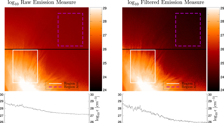
Figure 3. Total emission measure (top left panel) and total filtered emission measure (top right panel) exhibit similar features but differ by the diffuse background emission in high altitudes above the limb. The bottom two panels show emission measure plotted along the horizontal black cuts above. By removing the ambient contribution, the contrast is enhanced in the supra-arcade region and the resultant density is expected to better match the assumption of a simple slab structure.
Download figure:
Standard image High-resolution imageUltimately, we are interested in the plasma density; however, for the time being it suffices to focus on the electron number density, ne, which is assumed to be related to the column emission measure through

Here we have used d to indicate the (unknown) emission column depth of the supra-arcade fan. Without specifying d, we can still track the plasma evolution through the column depth normalized electron density,

from which the actual plasma density can later be extracted by assigning a value to d and converting from electron number to ion mass.
2.2. Continuity
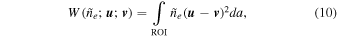
With (a proxy for) the density in hand, we may investigate the plasma velocity,  , through the continuity equation, which can be stated in terms of
  as
as

Here we have assumed that the column depth, d, is spatially and temporally invariant. The expression above relates the change in density to the divergence of  , which, like any two-dimensional (2D) vector field, can be expressed as the sum of irrotational and solenoidal components. Taking

the irrotational component must satisfy

from Equation (5). The fluid velocity is then given by

where  is, as yet, unspecified.
Since  is unconstrained by continuity, consideration of the electron density is only sufficient to partially specify the velocity; in order to fully determine the velocity, we must invoke an additional constraint. In an effort to incorporate all available information about the system, we turn to Fourier Local Correlation Tracking (FLCT), which provides a means for quickly estimating the apparent velocity of intensity features (Fisher & Welsch 2008). As with most optical flow solutions, FLCT assumes an advective evolution of the form

and the associated velocity field  is found through minimization of the residual in Equation (9), where I is the image intensity and is equivalent to ρ in our application. This assumption departs from the behavior of the continuity equation through exclusion of the term
  , which allows for the local depletion or enhancement of density features with no displacement of the overall structure. As such, the FLCT-derived velocity is nonconservative; therefore, while it does excel at characterizing the apparent motion of optical features (i.e., gradients), it is fundamentally inconsistent with the continuity equation.
Despite this limitation, the FLCT-derived velocity fields have the benefit of exhibiting much of the behavior that is apparent to the eye. We therefore choose the solenoidal contribution to Equation (8) such that the resultant velocity is as much like the FLCT-derived optical flow as possible, while still satisfying the continuity condition, as constrained through Equation (7). This is accomplished by developing a functional related to the variance of the density-weighted difference between the two velocities, integrated over the region of interest (ROI), i.e.,
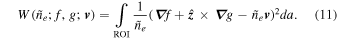
where da (=dx dy) is the differential area element in the image plane. By rewriting  in terms of its potentials, we find an equivalent form for the aforementioned functional:
Demanding that W be stationary under variations of g, with  , f, and
  held fixed, we can then choose g in order to minimize the value of this functional in each frame, with W guaranteed to be a minimum since no maximum value for the variance can exist.1
The Euler–Lagrange equation for g is then
held fixed, we can then choose g in order to minimize the value of this functional in each frame, with W guaranteed to be a minimum since no maximum value for the variance can exist.1
The Euler–Lagrange equation for g is then
Inspection reveals that the above expression is identical to the requirement that  . That is, the velocity field that differs the least from the FLCT-derived velocity and still satisfies continuity has a curl that is identical to that of the FLCT-derived velocity.
The right-hand side of Equation (7) was estimated by first smoothing the column emission measure in time using a three frame boxcar average, which helped to suppress fast-moving artifacts from the data, and then subtracting the smoothed value of adjacent frames. We then solved for f in the Fourier domain, where the solution and its Fourier transform,  , are given by

and

with f set to zero along the boundaries and  .
.
The dependence of Equation (12) on both  and
and  prohibits a simple inversion, and so a solution must be found through iterative relaxation. The algorithm that we used in determining the solution is as follows:
constructed given the current value of g = gi. Then, from Si we construct gs such that

Finally, gi+1 is given by

with R ≲ 0.5 controlling the rate and stability of convergence. Each solution for gs is found by solving Equation (16) in the Fourier domain, as with solutions for f, and the overall solution for g is said to have converged when the global average of the eccentricity between successive steps falls below a critical value of
This scheme appears to converge significantly faster than finite difference relaxation methods, likely owing to the fact that the intermediate solutions, gs, contain information about every pixel within the numerical domain (a feature of the Fourier transform), whereas for finite difference methods each pixel only receives information about its nearest neighbors. A representative example of the complete velocity inversion is shown in Figure 4.
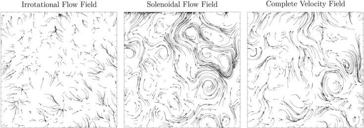
Figure 4. Contributions to  are given by
  (left panel) and
  (middle panel). Together they form the continuity consistent velocity field that most closely resembles the FLCT-derived optical flow (right panel).
Download figure:
Standard image High-resolution image3. DATA-ASSIMILATED FIELD TRANSPORT
We have outlined a method for obtaining the density and flow velocity within that portion of the fan with well-observed emission. The flows there, shown in Figure 4, have a qualitative appearance suggestive of non-negligible plasma β. That is to say, the forces generating those flows appear to demand pressure gradients in addition to the Lorentz force. In order to make this claim more rigorous, we will use the measured flows to infer the form of the magnetic field and then demonstrate that the resulting Lorentz force is insufficient to achieve the observed forcing of the plasma. We refer to this technique as a Data-Assimilated Field Transport (DAFT) model, since it is predicated on the idea of using observational data, which are assimilated into the model, to transport the magnetic field lines.
Outside the region with well-observed emission, which we will call the DAFT region, there is another region, in which the signal-to-noise ratio (S/N) for EUV emission is relatively low. For reasons that will become apparent, we refer to this as the Alfvén region. While the density inversion described in the previous section works well in the DAFT region and is largely insensitive to the details of the Alfvén region, the density and velocity within the Alfvén region are not well constrained by these methods. The location of the low-S/N cutoff is both spatially and temporally dynamic, so any rigid boundary that contains all of the interesting dynamics in the DAFT region and none of the Alfvén region would be difficult to treat. Therefore, rather than attempt to isolate only the DAFT region, we allow both regions to occupy portions of our data cube. As such, any method for inferring their coevolution must somehow account for their interaction.
Simultaneous treatment of both regions begins with the momentum equation and induction equation of ideal MHD:


where we have neglected viscosity, resistivity, and gravity. Since observations have provided the velocity in the DAFT region, which we refer to as  , we will use these equations to derive the pressure and magnetic field there. The velocity in the Alfvén region, called
  and not to be confused with the Alfvén speed, Va, is not constrained by observations and must therefore be derived, along with the magnetic field, using these equations. The result will be a composite velocity field,
  , combining these two regimes, and a magnetic field,
  , that spans the entire domain.
3.1. Composite MHD
Just as with the velocity treatment in Section 2.2, we assume that the magnetic field is inherently 2D and can therefore be written in the form of a flux function, φ, such that

where  is taken as a direction of symmetry, out of the plane. The uncurled form of the induction equation is then

Since  is fully specified in the DAFT region, any initial field configuration is sufficient to completely specify the magnetic field at all future times within that region. We need only choose the initial configuration that best describes the system.
The velocity in the Alfvén region will depend on the magnetic field and the interaction with the DAFT region, as well as the choice of boundary conditions at the edges of the domain. In the Alfvén region, we expect the pressure term to contribute little to the forcing of the plasma. Further, since the velocity is not constrained by observation, we cannot determine both the magnetic field and the pressure from Equations (19) and (22). We therefore rewrite the momentum equation for the Alfvén region in a form that will be dominated by Alfvénic waves:

By omitting the pressure and replacing the density with  , the Alfvén speed, Va, may be specified independently of the background magnetic field strength so that, when linearized and expanded about a smoothly varying equilibrium, as in the WKB limit, the fast magnetosonic wave mode naturally emerges with an isotropic wave speed, while the slow magnetosonic mode is suppressed. Note that in the case of propagation parallel to
  , the fast magnetosonic wave is degenerate with the shear Alfvén wave, hence the moniker Alfvénic.
In order to connect the DAFT and Alfvén regimes into a single solution, we use a weighted average for the velocity evolution. We define a Boolean mask, H, such that H = 1 where the S/N ≫ 1 and H = 0 where the S/N ≤ 1. H is also set to zero for a 10 pixel buffer along the edges of the numerical domain so that the observed velocities do not conflict with the boundary conditions. From inspection, the S/N scales with the emission measure, which falls off with height above the arcade, so the transition from H = 1 to H = 0 tends to occur on a band that extends from the upper left to lower right of the simulation domain, as seen in Figure 5.

Figure 5. In this image  (shown in red-yellow brightness) has been multiplied by H + 1 so that the DAFT region, where
  , is visibly enhanced relative to the Alfvén region, where
  . The black contour shows the
  level, indicating the shape of the transition band, which evolves from frame to frame as the density, and therefore the location of the S/N threshold, evolves.
Download figure:
Standard image High-resolution imageA selection function,  , is then developed by iteratively smoothing H while holding all of the zero values fixed.
  therefore satisfies the same requirements as H, but ramps progressively from 0 to 1 over a spatial scale of ∼10 pixels. The combined evolution of the velocity field everywhere in the numerical domain is then given by

with  determined as in Equation (23) and
  given by

For the 2011 October 22 event it was observed that the S/N of the filtered column emission measure (f) approaches unity as the signal drops below about 15% of the mean, which value was ultimately adopted for the threshold value of H.
This coupling of the DAFT region to the Alfvén region serves two purposes. First, it breaks up the behavior of the boundary conditions into two elements, with the Alfvén region serving as an intermediate layer. Since the physics of the Alfvén region and the details of the coupling are easily characterized, this introduces fewer artifacts than might be expected from an abrupt boundary. And since, as we shall see, the behavior in the Alfvén region is dominated by wave modes, its interaction with the boundaries on the exterior of the numerical domain is likewise simpler and better behaved than if the DAFT region were to abut those same boundaries. The second purpose for the coupling is to attempt to model how a highly dynamic supra-arcade structure might stimulate the evolution of the extended corona, which point we will return to in Section 4.
Given an initial configuration for the magnetic field, the aforementioned versions of the induction and momentum equations provide a prescription for advancing the system. It remains only to set the boundary conditions. At the bottom (sunward edge) of the domain we have chosen to anchor the field to the boundary. This is done to respect the assumption that the field lines emanate from a magnetically dominated region in the lower corona, which is unaffected by the motion of plasma in the supra-arcade region.
For the other three boundaries we choose a nonreflecting boundary condition.2 This is accomplished by setting the velocity at the boundary to be consistent with an outward-propagating, transverse, fast magnetosonic wave, as described by the linearized MHD wave equations. The associated wave eigenvector is given by
where  is the normal direction to the boundary and

is the component of the magnetic field perpendicular to the initial background field,  . Imposing this condition on the velocity at the boundary ensures that any outward-traveling, transverse waves will escape through the boundaries of the numerical domain, rather than being reflected as would be the case for Neumann, Dirichlet, or even mixed boundary conditions. So long as
  , this scheme performs well. It does, however, become unstable as the perturbation grows, owing to the nonlinearity of the system. We therefore use a weighted average based on the relative strength of the perturbation, with an open boundary condition employed in the limit that
  .
.
These boundary conditions complete the prescription for evolving the fluid velocity and magnetic field forward in time from an initial condition. Unfortunately, direct measurements of coronal magnetic fields are unavailable in the supra-arcade regions, where extrapolations are insufficiently resolved and polarimetry is photon starved. We must therefore infer, from inspection of the emission features, a likely initial field configuration. This is done by observing the alignment of spiky supra-arcade features and assuming that they are aligned with the large-scale orientation of the magnetic field. Then, since nothing depends on the overall magnetic field strength (as yet), the initial field configuration is taken to be a potential field, of arbitrary strength, whose field lines best coincide with the spiky arcade features that will later appear.
The initial condition, as well as several subsequent states of the system, can be seen in Figure 6. In the Alfvén region, Va has been set to 30 km s−1 in this example, in order to increase the apparent amplitude of transverse oscillations in the Alfvén region, which are difficult to distinguish as Va is increased. Of particular note are the pockets of low-density plasma that descend downward through the left-hand portion of the image domain, and the way the field lines move to accommodate the plasma motion. The transverse oscillations that have been observed along the edges of SADs have been previously characterized by Verwichte et al. (2005), and it seems likely that the corresponding motion of the magnetic field is related to this motion through the well-known equations of magnetohydrodynamics. Here, the coupling through the induction equation has been made rigorous. But to fully understand the system, we must also inspect the influence of the Lorentz force as it appears in the momentum equation; and for that we must attempt to infer the strength of the magnetic field.
Figure 6. Combined solution for the magnetic field and the velocity is depicted in four near-consecutive frames at 120 s cadence. Field lines are shown in green, and plasma density is shown in (log10) gray scale.
(An animation of this figure is available.)
Download figure:
Video Standard image High-resolution image3.2. Magnetic Field Strength
In the preceding sections we developed a solution for the evolving magnetic field without ever specifying the overall field strength. This was a consequence of the fact that the induction equation is independent of the overall strength of the magnetic field, as well as the imposed definition for the plasma density in the Alfvén region—the density there is proportional to  , so the momentum equation for that region is independent of
  . As such, the induction equation and the Alfvén momentum equation both depend only on the structure of the magnetic field. The only dependence on the strength of the magnetic field is in the momentum equation in the DAFT region, which we have avoided solving. However, if we suppose that the momentum equation that governs this region is balanced, then we may gain further insight by comparing the plasma acceleration to the Lorentz force and thereby estimating the contribution from the magnetic field.
Returning to Equation (19) for the evolution of  , the only unknowns are the global scaling for the density (i.e., d), the overall magnetic field strength, and the pressure. As with the continuity equation, the density may be written in terms of
  and d, while the Lorentz force can be expressed as the product of the overall magnetic field strength and a scale-free structure function,

Here we have taken the spatial and temporal mean of  to be one so that the definition for the magnetic field in Equation (21) gives the typical field strength as
  . Since the plasma pressure is unknown, we proceed by first taking the curl of Equation (19). The resulting expression depends only on the overall magnetic field strength, the column depth, and terms that are already known to us. That is,
where  is the typical ion mass, mp is proton mass, and 1.15 is the approximate ratio of protons and neutrons to unbound electrons in the solar corona so that the plasma density is given by

In order to achieve an exact balance in Equation (29), we would need to normalize the field strength to the line-of-sight depth independently for every pixel in every time step. However, since the structure of the magnetic field is already known, only the global field strength may be specified. Thus, the line-of-sight depth would have to be spatially and temporally variable, which is inconsistent with the assumptions made in Section 2.2. Equation (29) is therefore taken not as a local prescription but rather as a mean field normalization. That is, the line-of-sight depth is related to the typical magnetic field strength through

where the brackets imply averaging in space and time and we have used the shorthand notation for the advective derivative,  .
.
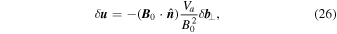
Typical values for the magnitude of the contributions to Equation (29) can be seen in Figure 7. In order to estimate the exact value of this normalization, we considered averages over only the interior of the DAFT region, where the Alfvén momentum equation makes no contribution. This resulted in an overall magnetic field strength of

where d = d6 × 103 km. Comparing this result with the findings of other authors, Savage et al. (2010) estimated the thickness of a similar fan structure in the so-called cartwheel flare of 2008 April 9 to be on the order of 5 × 10³ km. If this value is used for d, the corresponding magnetic field strength is ![$\sim 1.2\;G\sqrt[-4]{5}\approx 0.8\;G$](https://content.cld.iop.org/journals/0004-637X/819/1/56/revision1/apj522577ieqn49.gif) . Conversely, McKenzie (2013) performed a potential field extrapolation for the same 2011 October 22 event that we consider here and found that the typical magnetic field strength in the fan structure was in the range of 4–12 G for the potential field. Thus, our measured value, given the assumed column depth, is somewhat lower than previous estimates, but not unreasonably so.
. Conversely, McKenzie (2013) performed a potential field extrapolation for the same 2011 October 22 event that we consider here and found that the typical magnetic field strength in the fan structure was in the range of 4–12 G for the potential field. Thus, our measured value, given the assumed column depth, is somewhat lower than previous estimates, but not unreasonably so.
Figure 7. Distribution of values for the curl of the scale-free Lorentz force and the inertial response of the plasma are shown in the top and middle panels, respectively. The distribution of  , shown in the bottom panel, is found from the square of their ratio. A column depth of 103 km is assumed in every case.
Download figure:
Standard image High-resolution image4. RESULTS
From the previous section we have already estimated a normalization for the magnetic field strength in this event, which depends weakly on the column depth and is typically of the order a few G for column depths on the order of a few times 103 km. From this we can begin to estimate magnetic signatures that events such as this might be expected to produce. We shall focus on three aspects—namely, the temporal power spectrum of radiated Alfvén waves, the Poynting flux at various locations within the simulation domain, and the plasma pressure necessary to account for any forcing not consistent with the magnetic field.
4.1. Radiated Alfvén Waves
One advantage of the hybrid momentum equation is that we are able to simultaneously treat the evolution of both the highly dynamic plasma immediately above the arcade and the response of the plasma in the more extended corona. This allows us to address the question of how a magnetically dominated, slowly evolving extended corona might respond to being driven by a higher-density region with complex behavior involving the motion of magnetic elements and SADs.
In the model, this transition is handled by the selection function,  . In the majority of the domain
  has an integer value of either 0 or 1, but in the transition layer, where
  , a superposition of Equations (25) and (23) approximates the type of behavior that might be expected in a region where the pressure and density fall off rapidly and a highly dynamic region with nontrivial plasma pressure behaves as a driver for a more rarefied region, which responds by radiating energy away in the form of Alfvén waves.
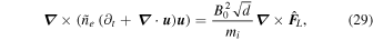
First, let us consider the Temporal Power Spectral Density (TPSD) of both the magnetic and velocity fields, averaged over two regions of interest (regions 1 and 2), corresponding to  (well within the DAFT region) and
  (well within the Alfvén region). The exact locations of regions 1 and 2 are indicated by the solid white and dashed purple boxes, respectively, in Figure 3. The TPSD for each of the fields in the ROI is given in terms of the Fourier transform of the windowed field, averaged over the ROI. That is, if

is the Fourier transform of the ith component of the magnetic field multiplied by a temporal window function, w(t), then the corresponding TPSD, averaged over some subregion Rj, is given by

For our analysis, we considered only the x-component of the velocity and magnetic fields, as it was observed that the behavior in y was identical. In practice, we applied a Hann window function for w(t), generated via HANNING.PRO from the standard IDL distribution.
In exploring the effect of varying the specified Alfvén speed in Equation (23), it was observed that a critical frequency arises in the TPSDs in region 2, above which frequency the TPSDs roll off and contain very little power. This frequency was found to correspond to the Alfvén crossing time of the transition band—that is, fcrit ∼ Va/λH, where λH is the characteristic width of the  transition—and we have hypothesized that it corresponds to an impedance matching issue of sorts. By setting Va = 103 km s−1, the critical frequency was pushed past the Nyquist frequency, and this artificial roll-off was eliminated from the TPSDs in region 2, at which point the spectra appeared to become independent of the choice of Alfvén speed. For this reason, all subsequent analysis is related to simulation runs with this choice of Alfvén speed.
Comparing the power spectra of the two fields in Figure 8, we find that while the velocity TPSD in region 1 is largely flat above frequencies of 10−3 Hz, the response of the magnetic field in this region shows that p[b,1,x] ∼ f−2. We attribute this to a fundamental aspect of the induction equation. Consider that, to first order, Equation (20) is equivalent to

where φ0 and φ1 are the equilibrium magnetic flux function and the associated perturbation, respectively. If we take the equilibrium field to be radial, as it was in the previous section, then this expression becomes

Then, because differentiation in the time domain is equivalent to multiplication by angular frequency (ω = 2πf) in the Fourier domain, we can write the spatial average of the Fourier transform of φ1 as

Figure 8. The temporal power spectral density of one component of the velocity and the corresponding component of the magnetic field are shown for each of the two regions (1 and 2) as solid red and dashed blue curves in the top and bottom panels, respectively. The dotted line indicates a power law of  in the case of the magnetic field and f−1 in the case of the velocity.
Download figure:
Standard image High-resolution imageApparently, if the spatial average of the Fourier transform of the perpendicular velocity field (uθ in this case) is vaguely “white,” then the induction equation will integrate it into a “pink” magnetic field spectrum. Of course, in a system with a momentum equation that continually responds to the changing magnetic field, this would likely be suppressed since uθ would itself be a function of φ1. But in region 1, where the velocity was derived with no dependence on the magnetic field, the noise within the velocity data is decoupled from the momentum equation. The induction equation treats the velocity noise as a source term, which is then integrated, and the result is a magnetic power spectrum that decays as a power law of the frequency.
To further understand the system, consider the general slope of the power spectra in region 2. Note the approximate coincidence of many of the peaks in the two spectra in the top panel of Figure 8. Also, from the bottom panel of the same figure we can see that the magnetic field in region 2 inherits most of its spectral profile not from the magnetic field in region 1, but rather from the velocity field in region 1. Apparently, while the magnetic field passes through the transition layer, it is, ultimately, the velocity field in the DAFT region that dictates the evolution of the Alfvén region.
Finally, we consider the relationship between the magnetic field and the velocity in the Alfvén region. Since Equation (23) contains no dependence on either ρ or p, only fast magnetosonic waves are expected in the Alfvén region. The fast magnetosonic eigenmodes for propagation parallel and perpendicular to  are given by


respectively, where  is the wavevector. Note that, regardless of
  , while the velocity perturbation is always perpendicular to
  .
.
Since the background magnetic field is constant in time, the power spectra for the two fields in this region should be proportional if the response is linear, which is not altogether obvious considering that Equation (23) is nonlinear in  . Inspection of Figure 9 shows that, indeed, with the exception of the extreme low-frequency end of the spectrum, the TPSDs of the two fields in the Alfvén region track almost exactly. The fact that the constant of proportionality is (almost exactly) Va/B0 is due to the fact that we have sampled, not
  and
and  , but rather
  and
and  , each of which contains contributions from both modes. The proportionality between these two components is therefore an average over transverse and compressional modes. But since each of those modes is related through Va/B0, so too is the proportionality between the sampled components of the velocity and the magnetic field. Therefore, we cannot claim that one mode contains more energy than the other.
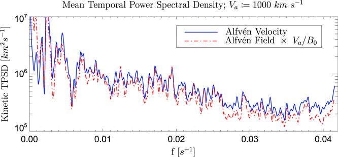
Figure 9. The temporal power spectral density of one component of the magnetic field and the corresponding component of velocity are shown for region 2 in dashed red and solid blue, respectively. The magnetic TPSD has been scaled by the ratio of the Alfvén speed and the background magnetic field strength.
Download figure:
Standard image High-resolution image4.2. Poynting Flux
Next, we considered the Poynting flux, defined for our purposes according to

Since the background magnetic field is given as a radial field, with its origin located just below the ROI (see Figure 6), we have chosen to parameterize the “outward” energy flux in terms of the radial component of the Poynting flux, Sr, defined consistently with the same coordinate system as used for the magnetic field. That is, escaping energy is quantified through

This estimation of the radial energy flux is shown in Figure 10 for a representative frame, approximately 15 minutes after the system is initiated. Note that within the DAFT region (especially within region 1) both positive (antisunward) and negative (sunward) energy fluxes are in evidence. However, near and above the transition layer (indicated by the two nested bands of solid black) the radiated energy is heavily dominated by positive flux, owing to the preference of the system to radiate energy into the lower-density, weaker field of region 2, and ultimately out through the nonreflecting boundary.
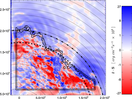
Figure 10. Radial Poynting Flux is depicted in the red-blue color table, with blue indicating outwardly radiated energy. The concentric black rings indicate successive radii, while the two bolt concentric rings indicate the contours of the  and r ≈ 2.0 × 10⁵ km levels in dashed and dot-dashed, respectively. The concentric contours that appear within the two circular dashed bands indicate different levels of
  , demonstrating the complexity and approximate location of the transition band where
  .
.
Download figure:
Standard image High-resolution imageTo further explore this behavior, we have divided the simulation domain into concentric regions of increasing radius, defined consistently with the initial magnetic field. These bands are depicted as the regions between concentric arcs in Figure 10. We then calculated the mean value for the Poynting flux in each band, as well as the total flux through each band. These are shown in Figure 11. For these estimates, a mean field strength of 1.2 G has been used, equivalent to a column depth of 103 km. Since the Poynting flux scales with the square of the magnetic field, these estimates are inversely proportional to the square root of the column depth.
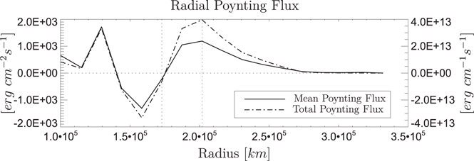
Figure 11. Mean and total Poynting fluxes through bands of successively larger radii are depicted by the solid curve (scale to left) and dashed curve (scale to right), respectively. The vertical dashed lines indicate the location of the r ≈ 1.7 × 10⁵ km and r ≈ 2.0 × 10⁵ km bands, which in turn indicate the locations of zero net radiated power and the peak value of the outward Poynting flux, respectively.
Download figure:
Standard image High-resolution imageFrom Figure 11 we see that, for a column depth of 103 km, the typical Poynting flux is on the order of 103 erg cm−2 s−1. If we instead assume a deeper column depth of 104 km, this value decreases by roughly a factor of three. And while there is a strong negative contribution below radii of approximately 1.7 × 10⁵ km, the net flux below 2.0 × 10⁵ km is quite small, and above that level the mean flux in each concentric band is positive definite and decays with radius, as would be expected for conservation of transmitted power.
The total flux through each band, multiplying the mean flux by the area of each band and then dividing by its radial width (an approximation of the arc length), demonstrates a similar behavior. And when we compared the details of where the radial Poynting flux becomes positive definite, we found a close correspondence to the  transition band, indicating that this layer behaves as a source surface for radiated Alfvén energy.
Unfortunately, since the arc length of each band decreases above radii of 2.0 × 10⁵ km, this does little to demonstrate whether power is conserved through successive bands.3
This may be due to imperfections in the nonreflecting boundary conditions, which can be seen along the edges of the numerical domain in Figure 10. However, if we take the peak value for the total flux and multiply by the estimated column depth of 103 km, we find that the upper bound for the radiated power from this region is approximately 4 × 10²¹ erg s−1, much lower than the energy budget of a typical solar active region (Tarr et al. 2013), but perhaps large enough to be detectable in the solar wind. This estimate of the total radiated power scales as  , so if the assumed column depth is increased to 104 km, the total radiated power is approximately 1.2 × 10²² erg s−1.
4.3. Pressure and Plasma Beta
Having scaled the magnetic field strength to the column depth, we may revisit the momentum equation, the divergence of which is
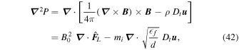
where the pressure, P, is given in terms of units of the magnetic field strength, i.e.,  . Since each term on the right-hand side of Equation (42) is already known, the plasma pressure is well constrained and Equation (42) can be solved through multiplication by
  in the Fourier domain using the same techniques as in Section 2, with the pressure gradients set to zero on the boundaries in order to give maximum freedom to the solution in the interior.
Because Equation (42) contains no zeroth- or first-order derivatives of P, the solution is only unique up to an additive harmonic function. That is, any function  satisfying
  can be added to P without affecting Equation (42), and we are forced to place an additional constraint on the system in order to find the pressure itself. We therefore choose to consider the smallest possible pressure that is everywhere non-negative within the DAFT region. This is found by first determining the minimum value of P from within region 1 and then subtracting this from the global value of P in every frame. This pressure, while not a unique solution to Equation (42), is the lowest possible thermal energy density that is physically meaningful without exploring the entire parameter space of harmonic functions that could be added to P. Figure 12 shows the magnetic and thermal energy densities (Pb and P), assuming a column depth of 103 km, as well as the plasma β, which is defined in the usual way:

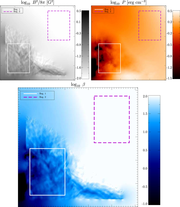
Figure 12. Two contributions to the total pressure (i.e., the magnetic energy density and thermal energy density) are shown in the top left and top right panels. The bottom panel shows the plasma β. The solid white box indicates a subregion corresponding to region 1 that is entirely within the DAFT regime, while the dashed purple box indicates a subregion of region 2, which is entirely in the Alfvén regime.
Download figure:
Standard image High-resolution imageWhile specifying the lowest value of the pressure within the DAFT region gives physical meaning to the pressure (i.e., the minimum possible thermal energy density), it has the unfortunate side effect of giving surprisingly large gas pressure values, and therefore β values, in the Alfvén region, high above the arcade. This would at first seem to be in conflict with our assumptions about the Alfvénic momentum equation in this region, per Equation (23). However, comparing Equations (23) and (19), we see that the simplified momentum equation of the Alfvén region assumes only that the pressure gradient is small. From the top right panel of Figure 12 it is clear that the pressure inversion described in this section correctly recognizes that the momentum equation is already balanced without contributions from  and therefore estimates the pressure in this region to be very smoothly varying, so as to contribute little to Equation (42), despite the relatively large pressure in that region.
On the whole, the plasma pressure that results from this calculation is typically less structured than the magnetic energy density—a natural consequence of being related through the Laplacian operator. And it is worth noting that since any change in the assumed column depth will rescale the overall magnetic field strength as B0 ∼ d−1/4, the plasma pressure and magnetic energy density both scale as  . Conversely, the plasma beta, which appears to be similarly structured to the magnetic field, is independent of assumed column depth and is, therefore, the only true measured value from this calculation. Histograms of each of these values are shown in Figure 13. Note that the peak value of the log10β distribution corresponds to a slightly higher value than would be found through comparison of the peaks of the other two distributions. This is a fundamental aspect of logarithmic distributions, that is, if n(β) is a distribution in β, then the corresponding logarithmic distribution is n(log10β) = βn(β), and the peak of this distribution is necessarily shifted to higher β values.
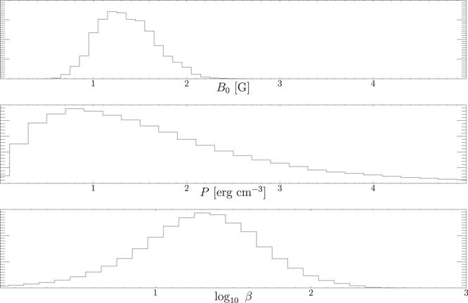
Figure 13. Histograms of the magnetic field strength, thermal energy density, and log10β are shown for the interior subregion, corresponding to region 1 in Figure 12. The log10β distribution is taken from the ratio of values in the upper two distributions.
Download figure:
Standard image High-resolution image5. DISCUSSION
This work represents an effort to estimate the otherwise poorly constrained plasma parameters in the supra-arcade region. We have used inversion techniques to estimate the plasma velocity and then ultimately evolve the magnetic field from some initial configuration. We then estimated the missing contributions to the momentum equation in the region where the observed plasma velocity was used. This allowed for normalization of the typical magnetic field strength to the assumed column depth of the supra-arcade fan. We found that for a column depth of ∼103 km the resulting magnetic field strength is ∼1.2 G and that this magnetic field strength scales inversely with the fourth root of the column depth.
We then went on to characterize the temporal power spectral density of both the velocity and the magnetic field. We found that the wave spectrum in the Alfvén region closely follows that of the velocity source in the DAFT region, independent of the f−1 scaling of the magnetic field in the DAFT region. We attribute this f−1 behavior to a decoupling of the induction equation in this region, which does not appear to influence the response of the Alfvén region. This estimate, while not directly applicable to estimates of solar-wind wave spectra, does provide insight into how the dynamics of low-lying coronal features might generate MHD waves that propagate into the extended corona and ultimately into the solar wind. Since the velocity TPSD in the Alfvén region inherits much of its shape from the velocity TPSD in the DAFT region, and the magnetic PSD in the Alfvén region mimics the corresponding velocity TPSD almost exactly, we suggest that one might be able to infer the spectrum of radiated Alfvén energy directly from observed velocities without making a detailed model of the magnetic field.
Considering the Poynting flux from this region, we find that where the pressure plays a strong role (in the DAFT region) the energy flux shows little evidence of a preferred direction, but as soon as the signals from the assimilated velocity reach the transition layer, there is a strong preference toward outwardly radiated energy. Further, we found that the typical Poynting flux just above the transition layer is of the order 103 erg cm−2s−1 and that integrating both along the arc length and the assumed column depth gives an estimate for the power radiating from this region in the range of 4 × 10²¹–1.2 × 10²² erg s−1.
Lastly, we attempted to characterize the plasma pressure in the DAFT region. For this we chose to report the smallest possible pressure that is consistent with the plasma evolution in each frame while still corresponding to a positive definite—and therefore physically meaningful—thermal energy density. In Figure 13 the distribution of possible values for the magnetic field strength and plasma pressure is shown, assuming a column depth of  , as well as log10β, which is independent of d. The peaks for these distributions are
  and P ≈ 0.8 erg cm−3, which correspond to a typical value of β ≈ 13. The typical value of log10β, which more aptly represents the range of possible behavioral regimes,4
has a peak at log10 β ≈ 1.3, corresponding to β ≈ 20.
and P ≈ 0.8 erg cm−3, which correspond to a typical value of β ≈ 13. The typical value of log10β, which more aptly represents the range of possible behavioral regimes,4
has a peak at log10 β ≈ 1.3, corresponding to β ≈ 20.
This estimate of β would seem to place the supra-arcade region firmly in the fluid-dominated regime; however, there are a few caveats. First, it should be noted that the distribution of values is rather broad, so that within the ROI there are pockets in which β could be significantly higher or lower. Moreover, the value that we have estimated is predicated on the assumption that the smallest possible value of p is zero and every other value is therefore larger than this value. Since the pressure is relatively complex and depends strongly on estimates of the magnetic field strength, which in turn depend strongly on the observed density and corresponding velocity inversion, it is reasonable to assume that the lowest value could be artificially low, which would bias every other value to be artificially high.
This could be further exacerbated by our inability to include additional forcing terms, such as microscopic turbulent processes or out-of-plane magnetic influences. For example, in the Savage & McKenzie interpretation of SADs, the retracting flux tubes penetrate the supra-arcade fan perpendicular to the surface normal. If such a structure indeed exists in this region, it is independent of the magnetic field that we have modeled, and any energy that said structure might deposit would necessarily appear as a pressure contribution, thereby biasing our result to artificially large pressure estimates and, correspondingly, artificially large β estimates. We therefore emphasize that these values should be considered not as a strict measurement, but rather as a likely upper bound.
Additionally, we suggest that while β may not be as high as we have estimated here (of the order of 10–20), our model has demonstrated that the supra-arcade region is certainly not consistent with a low-β environment; the transverse motions and swirling evolution of the magnetic field simply cannot be accounted for without the inclusion of some form of plasma pressure. We find it likely, therefore, that the supra-arcade environment corresponds to a plasma-β of the order of unity. This value has been employed in a number of numerical simulations of late (Cécere et al. 2012, 2015; Guo et al. 2014). Our own more recent work (Scott 2016) extends the efforts of Scott et al. (2013), showing that these results are also valid for β ≲ 1. In the coming years it will be important, therefore, to test each of these models against different β regimes; only in this way will we ever be able to truly pinpoint the energy distribution of the supra-arcade region and, simultaneously, explain the fundamental processes behind the evolution of supra-arcade features.
The authors would like to acknowledge the help of Joe Plowman for providing his DEM inversion software and for helping to understand its proper use and interpretation. We also thank Michael Freed, Kathy Reeves, Sabrina Savage, and Eric Priest for their contributions during private discussions, and we gratefully acknowledge the anonymous referee for their careful reading of the manuscript and helpful comments and suggestions. Finally, we acknowledge the generous funding of the National Aeronautics and Space Administration under contract NNM07AB07C, as well as the Living with a Star grant NNX14AD43G, without which this work would not have been possible.
Footnotes
- 1
Any assumed maximum value can be exceeded by globally increasing the value of
 .
. - 2
Both compressional and transverse fast magnetosonic modes are also expected within the Alfvén region, but the compressional mode propagates perpendicular to the background magnetic field and, therefore, parallel to the boundary in most cases.
- 3
These bands are inscribed within a square domain and typically meet the edge of the domain at an oblique angle.
- 4
The behavioral regime for 0 < β < 1 is as rich as for
. This is best captured by log10β, which maps the two regimes onto domains of equal size.

