Abstract
We show that viewing hypernetworks as polyhedral complexes represents a natural and expressive route towards their geometrization, that endows them with natural notions of curvature. We present both intrinsic and extrinsic methods towards equipping networks with such innate curvatures, and we dwell upon the most meaningful ones.
Original content from this work may be used under the terms of the Creative Commons Attribution 4.0 license. Any further distribution of this work must maintain attribution to the author(s) and the title of the work, journal citation and DOI.
1. Introduction
The present overview has been motivated by the confluence of two relatively recent developments in Network Science. On the one hand, on the mathematical side, one should note the introduction and even adoption in practice of discrete curvatures—mainly discrete Ricci curvature [45, 46, 73]. On the modeling side, there occurred the realization that network constitute popular means for representing pairwise relationships between elements in a complex system; therefore, the accent that was previously placed upon the separate entities constituting the network, that is, its nodes, is naive and, at least partially, contrary to the adopted model’s role. It should be noted, even at this stage, that the two motivations for our study are not unrelated and, in fact, the adoption and success of discrete Ricci curvatures stems precisely from the fact that they represent edge-based network measures, thus they constitute ideal tools for studying networks viewed as models of pairwise relationship. However, even such models soon proved to be insufficient for the representation of more complex relations. Indeed, many real-world complex systems, and especially those arising in social and biological sciences, higher-order interactions between three or more components also frequently occur. It has thus become quite common to consider not just networks, but also hypernetworks (as well as some other higher-order models, such as multilayer networks [35]). As far as the mathematical model adopted, given that graphs represent the essential mathematical tool for representing networks, it seems natural to adopt hypergraphs as the fitting analog for such higher-dimensional networks. However, while mathematically tempting, and certainly useful in many instances, this model does not capture a large class of networks that arise from real-life instances of substantial import.
Indeed, the convention adopted in Social Sciences is to add a (‘full’) triangle if there exist pairwise connections between three nodes, a tetrahedron if the same holds for four nodes, but only a quadrangle if the connections are circular, but not complete; etc. Some authors, however, do not ‘fill in the triangles’, and simply draw a triangle, quadrangle, etc with the implicit assumption that these represent two-dimensional faces—see figure 1, upper row, derived from [19], for such a modeling of higher-order contacts in the human genome. However, these n-tuples should be envisioned as ‘filled in’, as depicted in the middle row of the same figure.
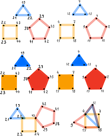
Figure 1. Emergence of n-tuples and hypernetworks in the human genome. Above: Left the most common 3-way, 4-way and 5-way intra-chromosome contacts within Chromosome 22; Right the most common 3-way, 4-way and 5-way inter-chromosome contacts from neonatal fibroblast (after [19]). Here the numbers denote the chromosome loci. Note that the authors draw triangles, quadruples, etc while presuming they are ‘filled in’ and we followed their original convention. Middle: the same n-tuples as above, as they should be conceived, that is as ‘filled in’ or ‘full’. Below: parts of the hypernetworks corresponding to the respective sets of n-tuples. (Note the double coloring, denoting common edges, in the configuration on the right, corresponding to the fibroblast data).
Download figure:
Standard image High-resolution imageHowever, in many instances—again, in particular in Biology—the process is streamlined by inserting a simplex whenever four nodes are interconnected (e.g. four genes are implied in a certain disease). (To be clear, since the data is obtained as correlation matrices, thresholding [50] and eventual filtration (even in the graph case) are employed in practice [55].) This clearly simplifies the geometrization process (albeit at the price of making it less expressive). Nevertheless, this easier approach is commonly used, since it is more convenient, for it needs no further understanding of all the pairwise interconnections in an n-tuple. Moreover, simplicial complexes are well known, classical structures, and in general quite well understood, thus using them as a basis for modeling presents definite advantages.
Consequently, also explains the reason why lately simplicial complexes—but not more general polyhedra—have started to be commonly considered in the study of hypernetworks. We favor the general polyhedra based approach, both because it allows for a better, more nuanced modeling of natural phenomena, but also because it is conducive to a more rich and interesting mathematical setting. Indeed, the reader should keep in mind that, in the discrete context, the poyhedral and simplicial categories are not equivalent, since subdivisions are not only not meaningful, but they are, in fact, not always possible, since adding arbitrary edges would ‘falsify’ the network. To wit, pairwise protein or gene interaction does not imply a common interaction. An even more intuitive illustration can be given using Social Networks: John might be a friend of Bob, and a colleague of Tom, while Tom and Bob might be acquainted, but this does not imply that John, Bob and Tom are coauthors of a paper. (We should also note that, there are problems that might arise, on a more theoretical level, even in the simplicial context, when performing subdivisions in tandem with embedding—see [12]). Nevertheless, given the fact that simplicial complexes are, as mentioned above, quite accepted in the field and, as they offer, moreover, the use of an extremely rich and beautiful mathematical theory, we adopt them as well, whenever they seem natural or important.
Remark 1.1. We should make it clear that we do not in anyway affirm that the polyhedral (simplicial) complex model is the ‘best one’ for hypernetworks, and certainly not the only one (for other significant models see, for instance, [21, 36]). In fact, we do believe that there exists no such optimal, absolute model, as each model has its own advantages and disadvantages, and, moreover, different types of hypernetwork can be better described using alternative hypernetwork models. Moreover, we are of the opinion that different models, shedding different lights on a problem, contribute to the better and more complete understanding of the modeled phenomena. (The classical example being that of the particle-wave duality in Quantum Physics). However, we do hold the opinion that the geometric model we adopt here has many advantages and expression force, by its very simplicity and intuitiveness, and we strive to present below as many facets of its modeling and analytic power.
Remark 1.2. While we do not explicitly specify, the discussion herein is essentially restricted to undirected networks (be they weighted or unweighted). True, many of the curvatures considered, and in particularly the Forman- and Ollivier–Ricci curvatures, as well as essentially all metric curvatures (that is, with the exception of curvature measures), have been extended to directed networks—see [68] and [66], respectively. To this end a choice of ‘properly’ oriented triangles should be made (see figure 2), which usually follows the one adopted by Alon et al [41], but which goes against traditional mathematical choice (and mathematical intuition as well) of cycles as ‘good’ triangles.
Moreover, the same convention can clearly be applied to higher-order cycles (quadrangles, pentagons, hexagons, etc). However, the ratio of polygons that admit an acceptable orientation decreases with the number of sides. Therefore, the resulting complexes are more ‘sparse’, that is they are more ‘graph-like’ as the lengths of cycles increase. The problem is further compounded if one attempts to assign an orientation to higher-dimensional cells. This stands again in stark contrast with the classical mathematical setting, where orientation can be axiomatically prescribed.
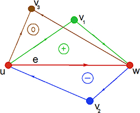
Figure 2. Oriented triangles and the sign they prescribe to the supporting edge  . Note that the ‘+’ sign is assigned to triangles concordant with transportation from u to w and the ‘−’ sign to transport in the opposite direction. Any other triangles in a directed network are discarded.
Download figure:
Standard image High-resolution imageHere we present two routes to such geometrization of hypernetworks, by regarding them as polyhedral complexes and, moreover, in a manner that attaches to them inherent notions of curvature. The first one, based on posets, on which we concentrate in section 2, gives an automatic method of generating simplicial complexes, in a manner that naturally endows them with a notion of Ricci curvature which, moreover, satisfies a fitting Gauss–Bonnet type theorem. The second approach, detailed in section 3, follows a natural path which, however, seems not to have been used before, namely to embed a network not into Euclidean, Hyperbolic or Hilbert space, as commonly done, but into a low-dimensional convex polytope, then consider the variety of discrete curvatures one can apply in the study of such an object or its triangulations. These range from some more classical ones, to modern ones, as well as to curvatures that one usually encounters in the study of graphs. We conclude this overview by some brief concluding comments.
2. Posets—the ‘Natural’ approach
We begin our excursus into hypernetworks curvatures with an approach that appertains to the second, more simplified, approach to generating hypernetworks that we discussed in the introduction. Moreover, it views hypernetworks as being hypergraphs, in the more restricted, traditional manner, that is adopting the definition in which vertices and hyperedges are considered, but no hypernodes as, in fact, many in the Complex Networks community do. (We shall return to the more general model in definition 2.2.) However, this perspective, based on the work of Bloch [8], presents two essential advantages: It provides a canonical method to construct a two-dimensional simplicial complex associated with a hypergraph, such that the vertices of the simplicial complex represent the vertices and hyperedges of the original hypergraph which, moreover, conduces to a natural way of defining the Forman–Ricci curvature of the vertices and the hyperedges as the scalar curvature of the associated vertices in the simplicial complex. As experiments on a wider range of real-life hypernetworks have shown [83], the Forman–Ricci curvature thus defined has a moderate to high absolute correlation with standard hypergraph measures such as eigenvector centrality and cardinality.
Remark 2.1. Before proceeding to present this approach in some technical detail, let us mention some relative advantages and disadvantages. On the applications side it has the drawback that, being combinatorial in nature, it is applicable only to unweighted networks. On positive side, Bloch’s version of Ricci curvature does satisfy the fundamental Gauss–Bonnet theorem. It should be noted that this is an important property, especially given the fact that the original Forman–Ricci curvature as defined in [24] does not satisfy a Gauss–Bonnet type theorem. This follows for a rather unexpected result of Forman (itself an extension to dimension two of a result of Lohkamp [37])—see [24], theorem 7.2—that states that given a combinatorial n-manifold M,  , there exists a finite subdivision
  of M such that
  for all edges e of
  . Thus, given the identity between Gauss and Ricci curvatures in dimension 2, the impossibility of a Gauss–Bonnet theorem for Forman–Ricci curvature in this dimension follows immediately.
Let us remark also that the existence of a Gauss–Bonnet type formula is not solely of theoretical import, given that it allows us to define gauge (or model) networks, which facilitates the study, through the Ricci flow, of the long-time evolution of hyper-networks, not just of networks [81].
We begin by reminding the reader the definition of the type of structure we study.
Definition 2.2 (hypernetworks). We define a hypernetwork as a hypergraph  with the hypernode set
  consisting of set of nodes, i.e.
  ,
,  ; and hyperedges
  , the hyperedge set of
  , the connecting groups of nodes/hypervertices.
Note that it is natural to view each hypervertex as a complete graph (or clique) Kn, which in turn is identifiable with the (1-skeleton of) the standard n-simplex.
Remark 2.3. Note that in [70] we have employed a somewhat more general, but also less common, definition of hypernetwork, where hypervertices where not viewed as complete graphs, thus allowing for the treatment of hypernetworks as general polyhedral complexes, not merely simplicial ones, as herein.
2.1. Posets
We briefly summarize here the minimal definitions and properties of partially ordered sets, or posets that we need in this section. In doing this, we presume the reader is familiar with the basic definition of posets.
Definition 2.4 (coverings). Let  be a poset, where
  denotes the partial order relation on
  , and let
  be elements of
  . We say that p covers q if p > q and there does not exists
  , such that
  . We denote the fact that p covers q by
  .
.
While a variety of examples of posets pervade mathematics, the basic (and perhaps motivating) example is that of the set of subsets (a.k.a. as the power set)  of a given set X, with the role of the order relation being played by the inclusion. Given the common interpretation of networks, the identification with hypernetworks with a subset of
  is immediate.
Definition 2.5 (ranked posets). Given a poset  , a rank function for
  is a function
  such that
- (1)If q is a minimal element of
 , then ;
 - (2)If, then . A poset is called ranked if there admits a rank function for . The maximal value of is called the rank of , and it is denoted by .





Note that in the definition of ranked posets we essentially (but not strictly) follow [8] and, while other terminologies exist [54, 74], we prefer the one above for the sake of clarity as well as of concordance with Bloch’s paper.
Let us note that if a poset is ranked, than the rank function is unique. Furthermore, if  is a ranked poset of rank r, and if
  , we denote
  , and by Fi the cardinality of
  , i.e.
  .
.
Again, as for the case of posets in general,  represents the archetypal example of ranked posets, thus hypernetworks represent, in essence, ranked posets, a fact which is essential for the development of the main idea of this section.
Remark 2.6. Many of the hypernetworks arising as models in real-life problems are actually oriented ones (see, for instance [67, 70]). For these the poset structure is even more evident, as the order relation is emphasized by the directionality. If, moreover, there are no loops, the resulting poset is also ranked.
2.2. Simplicial complexes and the Euler characteristic
As for the case of posets, we do not bring the full technical definition of a simplicial complex, but we rather refer the reader to such classics as [30] or [56].
Given a poset  , there exists a canonical way of producing an associated ordered simplicial complex
  , by considering a vertex for each element
  and an m-simplex for each chain
  of elements of
  . See figure 3.
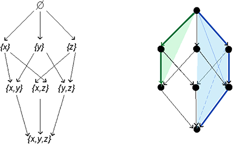
Figure 3. Left: the Hesse diagram of the poset of the subsets of the set  ordered by inclusion (left).
Right: the hypernetwork associated to it with it, with two elements of the simplicial complex associated to it, namely a triangle corresponding to a length two path depicted as the thick green line and a tetrahedron corresponding to a length three path depicted as the thick blue line.
ordered by inclusion (left).
Right: the hypernetwork associated to it with it, with two elements of the simplicial complex associated to it, namely a triangle corresponding to a length two path depicted as the thick green line and a tetrahedron corresponding to a length three path depicted as the thick blue line.
Download figure:
Standard image High-resolution imageSince in the present paper we considered only finite hypernetworks/sets, we can define the Euler characteristic of the poset  as being equal to that of the associated simplicial complex
  , i.e.

Note that this definition allows us to define the Euler characteristic of any poset, even if it is not ranked, due to the fact that the associated simplicial complex is naturally ranked by the dimension of the simplices (faces).
However, if  is itself ranked—as indeed it is in our setting—than there exists a direct, purely combinatorial way of defining the Euler characteristic of
  that emulates the classical one, in the following manner:

2.3. Forman curvature
Robin Forman introduced in [24] a discretization of the notion of Ricci curvature, by adapting to the quite general setting of CW complexes the by now classical Bochner–Weizenböck formula (see, e.g. [32]). We expatiated on the geometric content of the notion of Ricci curvature and of Forman’s discretization in particular elsewhere [57], therefore, in order not to repeat ourselves too much, we refer the reader to the above mentioned paper. However, let us note that in [57] we referred to Forman’s original notion as the augmented Forman curvature, to distinguish it from the reduced, one-dimensional notion that we introduced and employed in the study of networks in [73].
While in general  and
and  do not coincide, they are identical in the case of CW complexes, thus in particular for polyhedral complexes, hence a fortiori for simplicial complexes. In particular, we shall obtain the same Euler characteristic irrespective to the model of hypernetwork that we chose to operate with: The poset model
  , its associated complex
  , the geometric view of posets a simplicial complexes that attaches to each subset of cardinality k, i.e. to each hypervertex a k-simplex, or the more general polyhedral model that we considered in [70]. It follows, therefore, that
The Euler characteristic of a hypernetwork is a well-defined invariant, independent of the chosen hypernetwork model, and as such captures the essential topological structure of the network.
Here we shall concentrate, for reason that we will explain in due time, on the subcomplex of  consisting of faces of dimension
  , that is to say, on the 2-skeleton of
  . In particular, we shall show that
  is not just a topological invariant, it is also closely related, in this dimension, to the geometry of
  .
.
While Forman’s Ricci curvature applies for both vertex and edge weighted complexes (a fact that plays an important role in its extended and flexible applicability range), we concentrate here on the combinatorial case, namely that of all weights (vertex as well as edge weights) equal to 1. In this case, Forman’s curvature, whose expression in the general case [24] is quite complicated, even when restricting ourselves to two-dimensional simplicial complexes [57], has the following simple and appealing form:

Here t2 denotes triangles and e edges, while  denotes parallelism, where two faces of the same dimension (e.g. edges) are said to be parallel if they share a common ‘parent’ (higher dimensional face containing them, e.g. a triangle), or a common ‘child’ (lower dimensional face, e.g a vertex), but not both simultaneously. (See figure 4 for an illustration).
Remark 2.7. For ‘shallow’ hypernetworks, like the chemical reactions ones considered in [67], both Forman Ricci curvature and especially the Euler characteristic are readily computable but also, due to the reduced depth of such hypernetworks, rather trivial. This important but quite specific example illustrates the fact already mentioned above that the chosen hypernetwork model, suited to a certain application, can also limit the scope of meaningful computations.
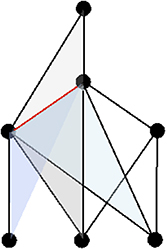
Figure 4. The four triangles (2-faces) adjacent to an edge (in red) in a small network. Thus, by Formula (3), the combinatorial Forman–Ricci curvature is  .
.
Download figure:
Standard image High-resolution image2.4. The Gauss–Bonnet formula
In the smooth setting, there exists a deep connection between curvature and the Euler characteristic, that is captured by the classical Gauss–Bonnet formula (see, e.g. [32]). While the Forman Ricci curvature, as initially defined in [24] does not, unfortunately, satisfy a Gauss–Bonnet type theorem, since no counterparts in dimensions 0 and 2, essential in the formulation of the Gauss–Bonnet theorem, are defined therein. However, Bloch defined these necessary curvature terms and was thus able to formulate in [8] an analogue of the Gauss–Bonnet theorem, in the setting of ranked posets. While in general the one dimensional curvature term has no close classical counterpart, in the case of cell complexes, and thus of simplicial complexes in particular, Euler characteristic and Forman curvature are intertwined in the following discrete version of the Gauss–Bonnet theorem (in which the notation accentuates the fact that in the simplicial case only triangular 2-faces appear):

Here R0 and R2 denote the 0-, respective two-dimensional curvature terms required in a Gauss–Bonnet type formula. These curvature functions are defined via a number of auxiliary functions, as follows:

where  are the aforementioned auxiliary functions, which are defined in the following simple and combinatorially intuitive manner:

Remark 2.8. The introduction of the combinatorial curvature functions (and especially those in dimension 0 and 2, which have no classical counterpart in Forman’s primary paper, in contrast with R1 which coincides  ) is the tool that allowed Bloch to obtain [8] an analogue of the Gauss–Bonnet theorem in the setting of ranked posets.
Since we only consider only triangular 2-faces, the formulas for the curvature functions reduce to the very simple and intuitive ones below:

where  denotes, conforming to the canonical notation, the degree of the vertex (or rather hypervertex) v, i.e. the number of its adjacent vertices.
From these formulas and from the general expression of the Gauss–Bonnet formula (4) we obtain (see [83]) the following combinatorial formulation of the noted formula in the setting of the two-dimensional simplicial complexes:

or, after taking into account also formulas (3) and (4):

Remark 2.9. Formula (4) and its variations allow for study the long-time behavior of evolving (hyper-)networks via the use of prototype networks of given Euler characteristic [81] by combining it with a properly adapted Ricci flow. This allows us to asymptotically simplify a network and reduce it to its essentials and predicting its evolution according to its Euler characteristic (inferred through the Gauss–Bonnet theorem). Unfortunately, while some experiments on small to medium sized experiments were performed [6], at this point in time, truly large scale implementation of this idea is still pending.
3. The embedding approach
The methods and problems considered so far relate to networks curvature as an intrinsic notion. While this approach, namely of viewing networks as geometric objects in their own right is certainly the deeper one and the ‘correct’ one to follow in the long run, considering networks as objects embedded in a standard ambient space is also natural and perhaps more intuitive. Indeed, it is a direction which, as we have already pointed out in above, was prevalent for a long time in the geometric study of graphs and networks (see, e.g. [11]). It is, therefore, only natural to consider it as well, especially so since, in truth, it allows us to introduce in a simple and intuitive manner, a number of pertinent curvature measures on a network/graph. Moreover, the ambient space is conceptually an easy one to grasp, namely a convex polytope. Additionally, there exist (at least) two different methods of obtaining such an embedding:
3.1. The embedding methods
3.1.1. Perles approach
The first embedding technique is perhaps the simpler, more ‘self contained’ one and that, furthermore, produces a highly symmetric ambient polytope. The basic idea is to realize the graph—with its (geo-)metric structure—as part of the 1-skeleton of a manifold (in fact, surface). The starting point is the following important observation due to Perles:
Theorem 3.1 (Perles [34, 47], proposition 19.2.3). Every graph is the spanning subgraph of a 4-polytope P4.
More precisely, P4 is the cyclic polytope and the embedding is realized by considering V points on the momentum curve  and V different values for t, e.g.
  . Recall that
Definition 3.2. A cyclic d-polytope is the convex hull of a set of n ( ) points on the moment (or momentum) curve in
  , that is
  .
.
Also, using a finite number V of values for t allows us to set the abstract definition above in a concrete, discrete setting for our purposes. Furthermore, by considering different V’s one can explore different realizations of a given graph (even though, the natural choice is the minimal one, that is in this specific case, V = 5).
Moreover, one has the following generalization of Whitney’s theorem (see, e.g. [34]):
Theorem 3.3. d-polytopes are determined by their  -skeletons.
Remark 3.4. For simplicial polytopes this result can be improved as follows:
Theorem 3.5 (Perles [47], see also [34]). Simplicial d-polytopes are determined by their  -skeletons.
However, this result presents no advantage in our case, given that d = 4.
These results are extremely important in our context, since they demonstrate that, even though formally one studies graph embeddings in P4, we have transformed the problem, from one concerning the geometry of graphs, to one concerning the one of two-dimensional simplicial complexes M2 (the ideal case, being, of course, that of M2 being a PL surface (simplicial 2-manifold). whose discrete curvature are, by now, classical and rather well understood. This is especially relevant, in particular, for the various discrete Ricci curvatures (which we shall discuss in some detail below), since they are determined by the 2-skeleton.
3.1.2. Tight span approach
The second embedding method produces a less simple and symmetrical structure, yet it makes appeal to a more standard construction, stemming, it would seem, from the classical Kuratowski embedding. For the sake of completeness, we remind the reader its definition.
Definition 3.6 (Kuratowski embedding). Let (X, d) be a metric space. Then

where

is called the Kuratowski embedding (of (X, d)).
Namely, one can consider the tight span  [5, 20] (also known as the injective envelope [31]) of a network
  viewed as a metric space, which is defined as follows:
Definition 3.7. Let  be metric spaces. A mapping
  is called an injective envelope of X if the following hold:
- (1)E is an injective metric space;
- (2)e is an isometric embedding;
- (3)There exists no injective proper subspace such that ;


Definition 3.8. A metric space (X, d) is called injective if for any metric space  , and any
  , any mapping
  , such that
  , for all
  , can be extended to a mapping
  satisfying the same no dilation condition as f.
Remark 3.9. Any metric space has an injective envelope which, moreover, is unique up to isometry (see [31], theorem 2.1).
This construction can be further refined by considering the secondary fan of the second hypersimplex  and its triangulation Δ, which represents the dual of the polyhedron
  , whose complex of bounded faces (see [39]) is precisely
  —see [13]. We bring here the definitions of the notions mentioned above, which might be less than familiar to some of the readers.
Definition 3.10. A (complete) fan is a convex set  of pointed polyhedral cones in some
  , such that
  .
.
Given a polytope  , the normal fan
  of P, contains, for each face
  , the collection CF of all the vectors
  , such that the linear function
  on P is minimized by all the points
  .
.
Recall that
Definition 3.11. Given a polytope  , the pointed (polyhedral) cone
  associated with P is the cone spanned by the points
  .
.
(For further details, see [27].)
Definition 3.12. The hypersimplex  is the convex hull of the binary vectors of length n that have precisely k components equal to 1.
(For further details, see [13].)
Remark 3.13. While the first method produces, as already mentioned, a more symmetric and simple construction, its caveat resides in the fact that is purely combinatorial in nature, as opposed to the tight span approach, which, by its very definition, intrinsically takes into account the network metric.
It is important to note that, given that this represents a convex body construction, at least as far as the first embedding method is concerned, it is viable from a computational viewpoint. Moreover, by passing to the Schlegel diagram1, we are reducing the problem to that of defining notions of curvature on (part of) the 1-skeleton of a three-dimensional convex manifold. It follows, therefore that it is in fact possible to graphically represent (schematically) the considered polytope, which represents a clear advantage in any empirical study in this direction. Even comparing the local embedding curvatures results according to [60] would represent, at this point, an interesting, if incipient step forward.
3.2. The innate curvatures
Having (convexly) embedded the given (hyper-)network into a polytope, with any of these two methods (and even better, by using both of them and comparing the results), one can endow the (hyper-)network (be it perceived of having hypervertices or not) and its embedding polytope with a plethora of curvature measures defined originally on piecewise-flat (and, more generally, PL) manifolds/complexes. Among these, one should consider:
3.2.1. The Lipschitz–Killing curvatures
The first type of discrete curvatures that we shall consider is stemming from Physics, more specifically from General Relativity. More precisely, it roots reside in a paper of Tullio Regge [51] (see also [52]). His goal was to produce a discrete, computationally feasible approach to Cosmology (namely for the determination of the solution of the Einstein field equations Einstein field equation), and his approach is now known as the Regge Calculus Regge Calculus. Cheeger, Müller and Schrader first sought to fully solve this problem from a mathematically stand point in [15], and brought the complete solution in [16]. To this end, they made appeal to a generic class of curvatures, which represent the focus of the present section.
We begin directly with the following technical definition:
Definition 3.14. Given a Riemannian manifold Mn, the Lipschitz–Killing curvatures of Mn are defined as follows:


where  are the curvature2-forms curvature form and ωkl denote the connection forms connection form, and they are interrelated by the structure equations:

where  is the dual basis of
  . Moreover, the integral
  is also known as the integrated mean curvature integrated mean curvature (of order j).
(For missing technical terms, see [16], as well as [18, 32].)
Remark 3.15. While the expression (11) above might appear daunting (and rightly so!...), in low dimensions Lipschitz–Killing curvatures are, in fact, quite familiar:  volume and
  scalar curvature. Moreover,
  Gauss–Bonnet–Chern form Gauss–Bonnet–Chern form, (for
  ).
).
We also have the following expression of the Lipschitz–Killing curvatures Lipschitz–Killing curvatures:

where  ,
,  denotes the
  -dimensional Hausdorff measure Hausdorff measure, and where the symmetric functions Sj are defined by:

 being the principal curvatures—see e.g. [38].
Remark 3.16. Formula (13) above shows why the Lipschitz–Killing curvatures are also called the total mean curvatures (and the ‘Sj’-s are called the mean curvatures (of orderj). It also suggests a quite direct method of obtaining a local (point-wise) version.
In a similar manner (but technically slightly more complicated), one can define the associated boundary curvatures (or mean curvatures mean curvatures) Hj which are curvature measures on  : let
: let  be an orthonormal frame for the tangent bundle
  of Mn, such that, along the boundary
  , en coincides with the inward normal. Then, for any
  , we define

where


and

These curvature measures are normalized by imposing the condition that:

for any flat  .
.
Remark 3.17. As expected, in view of the similar elucidation of the Lipschitz–Killing curvatures, the low dimensional boundary curvatures also have quite familiar interpretations:  area boundary,
  mean curvature for inward normal (as expected given the generic names for these Hj-s), etc.
The disconcerting formulation of the Lipschitz–Killing curvatures appears to leave very little chance for them to be applied in any concrete context. However, they can be expressed in terms of dihedral angles (see [16] for the proof), thus making them applicable in a variety of practical instances (as are other notions of discrete curvature that we shall discuss in detail in the following sections). More precisely, we have the following formula:


Here  denotes the (internal) dihedral angle. While intuitively simple, the formal definition of this notion requires some technical preliminaries. (For an alternative definition, see [72] IV. 2, IX. 15).
Definition 3.18. A simplicial cone  , is the set
  , where Hj are open half spaces in general position, such that
  . The set
  is called a spherical simplex.
Definition 3.19. Consider the simplices  , and let
  . The normal cone normal cone is defined as
  , where
  denotes the ray through x and base-point p. The spherical simplex
  associated to
  is called the link of σk in τm (see figure 5).
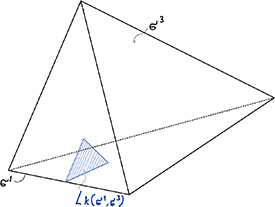
Figure 5. The link  of the simplex σ1 in σ3, identified with the set
  , for sufficiently small ε (after [16]).
Download figure:
Standard image High-resolution image(Note the slight change of notation for the link in this setting.)
Remark 3.20.  does not depend upon the choice of p.
We are now ready to formally define the notion of dihedral angle, as follows:
Definition 3.21. The (internal) dihedral angle  of σ in τ is the normalized volume of
  , where the normalization is such that the volume of
  equals 1, for any
  .
.
Before passing to the next relevant discrete curvature, let us notice that expressions similar to (19), but more complicated, exist for the boundary curvatures Hj—see [16]. Note that  and, in the case of PL manifolds, they represent the contribution of the
  -dimensional simplices that belong to the boundary. On a practical note, let us also remark that, since
  for j odd, and since R4 is just the volume, the only interesting L–K curvature in our setting is R2, that represents scalar curvature.
Remark 3.22. Beyond their motivating application to Regge Calculus, the Lipschitz–Killing curvatures are also important in probability—see, e.g. [1].
3.2.2. Glickenstein’s curvatures for piecewise-flat manifolds
In [25] and [26], Glickenstein introduced piecewise-flat versions of scalar and sectional curvature for PL (or, rather, piecewise flat) 3-manifolds. The simplest of them is a fitting version of scalar curvature at a vertex vi, defined as

where αijkl denote the solid angles at vi of the tetrahedra Tijkl (incident with vi). Note that αijkl can be computed using the relevant dihedral angles of Tijkl, namely

where βijkl denotes the dihedral angle of Tijkl, along the edge eij.
He also introduced—even in the case when the manifold is endowed with a metric—an edge curvature, which could be compared, in the sense, with our Forman–Ricci curvature, defined as

where lij denotes the length of the edge eij.
The geometric interpretation of this quantity is due to Regge [51], more precisely  is viewed as discrete (PL) version of parallel transport around the edge eij.
Another interpretation is due to Cheeger et al [16], who views this as the analogue of sectional curvature or rather of the (Riemannian) curvature operator.
The version of scalar curvature given by (22) is the one used in [25]. However, a more refined version is introduced in [26], namely

where dij denotes the weight of the directed edge  . Thus, even if obtaining it by going through the complication of embedding the given graph (combinatorially) into the 1-skeleton of the cyclic polytope and making appeal to its two-dimensional cells, this formula allows us define a theoretically sound and probably feasible, from a computational viewpoint, version of scalar curvature. (For an older, related approach to sectional curvature see Stone [75]).
The dual  to an edge
  is a surface which goes through
  for any tetrahedron T containing
  , and is perpendicular to
  .
.
A rather recent alternative approach, focusing on practical computations and also motivated by the Regge Calculus is that of Alsing, Miller and their collaborators [2, 3, 40]. In their thorough program they introduced simplicial Riemann and Ricci tensors, as well as Ricci scalar and sectional and scalar curvatures. While we do not present here the intricacies of their simplicial tensors, we very briefly bring below their definition of sectional, Ricci and scalar curvatures.
Definition 3.23. Let  an edge in a PL simplicial complex. Then the three essential types of curvature are defined as
- (1)The sectional curvature of e is defined aswhere the sum is taken over all the edges that share a common vertex with e (see figure 6); and where Ae denotes the dual Voronoi area [3, 40, 51] of the edge e, εe represents the deficit areas [3, 40, 51] of edge e, and θi is the angle between the edges e and ei (again, see figure 6).
- (2)The Ricci (scalar) (as it is called by Alsing and Miller) curvature of e is given bywhere denote the scalar curvatures of the vertices , respectively, and where
- (3)






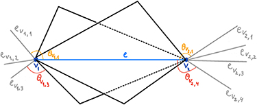
Figure 6. The edges and angles appearing in the definition of Alsing and Miller’s simplicial curvatures.
Download figure:
Standard image High-resolution image3.2.3. Stone’s Ricci curvature
In [76, 77] Stone developed a combinatorial Ricci curvature for cell complexes and proved that it satisfies the mandatory, for any notion of Ricci curvature, version of Bonnet–Myers theorem. His approach is based on developing PL variational (Jacobi) fields. He proposes, in fact, two formulas for the Ricci curvature of a cell complex.
The first formula is obtained by passing to the dual complex. The Ricci curvature at the vertex v (in the dual complex, if starting with a simplicial one) in the direction  is to be taken as the total defect of these
  cells, as follows:

where  denotes the length (combinatorial or metric, depending on the respective setting) of the cell
  (see figure 7).
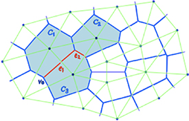
Figure 7. Part of the simplicial complex  and its dual cell complex
  . The (variational) Jacobi field given by
  cells (n = 2), in the direction
  , at the vertex v0 is emphasized .
Download figure:
Standard image High-resolution imageIt is important to underline the fact that, while apparently less intuitive, this approach is, in fact, more practical for or goals, since it allows computation of Ricci curvature directly, without first constructing the simplicial complex—see [28]. It represents, therefore, the approach that allows for the computation (again, directly) of the Ricci curvature for metric complexes, thus, eventually, for a fitting Ricci curvature for weighted graphs.
The Ricci curvature of the original (simplicial) complex is given by the following formula:

where  are faces of σ, and where
  denotes the number of n-simplices α, such that
  .
.
In the most relevant case for us, i.e. the two-dimensional case, the simplices βj are 0-dimensional, i.e. vertices, and  is just the number of 2-simplices having βj as a common vertex, hence
  represents nothing but the total combinatorial defect at these
  vertices. (See also [28] for the similar interpretation of
  ).
).
Note again that this apparently more direct approach is less intuitive than the one based on dualization, since it defines Ricci curvature at a simplex, in the direction of the difference of two simplices of lower dimension (faces), rather than at a vertex, thence it represents a somewhat counterintuitive discretization of the Riemannian case.
Returning to the definition of Ricci curvature for simplicial complexes: Given a vertex v0, in the dual of a n dimensional simplicial complex, a direction at v0 is just an oriented edge  . Since, there exist precisely n 2-cells,
  , having e1 as an edge and, moreover, these cells form part of n relevant variational (Jacobi) fields (see [76]), the Ricci curvature at the vertex v, in the direction e1 is simply

Observe that the index ‘i’ in the definition (28) above runs from 1, and not from 2, as expected judging from the classical (smooth) setting. This is due to the fact that we defined Ricci curvature by passing to the dual complex, with its simple but demanding (so to say) combinatorics.
Remark 3.24. Note that we followed [76] only in determining the variational fields, but not in his definition of Ricci curvature.
3.2.3.1. Metrization of Stone’s approach
Stone’s approach to discrete Ricci curvature is a purely combinatorial one. It is, however, clearly desirable to extend it to metric graphs, thence rendering it applicable to weighted networks. To determine—using solely metric considerations—the sectional curvatures  of the cells
  , we shall make appeal to the (modified) Wald curvature KW. To this end we begin by first defining metric quadruples:
Definition 3.25 (metric quadruple). Let (M, d) be a metric space, and let  , together with the mutual distances:
  . The set Q together with the set of distances
  is called a metric quadruple.
Remark 3.26. The following slightly more abstract definition can be also considered, one that does not make appeal to the ambient space: a metric quadruple being a 4 point metric space, i.e.  , where the distances dij verify the axioms for a metric.
Before being able to pass to the next definition we need to introduce some additional notation: Sκ denotes the complete, simply connected surface of constant Gauss curvature κ (or space form space form), i.e.  , if κ = 0;
  , if κ > 0; and
  , if κ < 0. Here
  denotes the sphere of radius
  , and
, and  stands for the hyperbolic plane of curvature
  , as represented by the Poincaré model of the plane disk of radius
  .
.
Definition 3.27. The embedding curvature  of the metric quadruple Q is defined to be the curvature κ of the gauge surface Sκ into which Q can be isometrically embedded—if such a surface exists.
Remark 3.28. In the present setting we cannot discuss the intricacies and pathologies of the definition above, thus we refer the reader to, e.g. [9] or, for a more readily accessible source, [62].
We can now bring the desired definition of the embedding curvature of cells, thus introducing the final necessary ingredient for the metrization of Stone-Ricci curvature given in (28).
Definition 3.29. Let  be a cell with vertex set
  . The embedding curvature embedding curvature
  of
of  is defined as:

Remark 3.30. (1) Evidently, the definition above presumes that cells in the dual complex have at least 4 vertices. However, except for some totally degenerate (planar) cases, this condition always holds. (Moreover, it can be easily corrected by truncation of the problematic vertices).
(2) Obviously, one can use the same method as above to compute the Ricci curvature (of  ), according to Stone’s original approach for determining directions in cell complexes.
Remark 3.31. While, unfortunately, no truly relevant applicative results are available yet, the metric Stone-Ricci curvature [28] and its associated flow [61] satisfy many of the essential theorems and convergence properties of the classical [17, 29] as well as combinatorial [17, 76, 77] notions. Thus the metric Ricci curvature and flow bridges the gap between smooth and combinatorial notions via a computational approach to the Alexandrov comparison curvature. (For this notion and its connection to the Wald metric curvature the reader is referred to [61] and the bibliography therein, since this discussion extends far beyond the scope of this paper).
Remark 3.32. The theoretical advantages of the metric metric approach to discrete Ricci curvature expounded above are counterbalanced by the difficulty of actually computing the metric Stone-Ricci curvature, due to the transcendental functions included in its definition (see [79, 80] and, for more accessible sources, [28, 61]).
3.2.4. Ollivier’s Ricci curvature
The inclusion of Ollivier’s Ricci curvature among the curvatures innate to the Euclidean space might surprise the reader, given that it is an archetypic intrinsic curvature for graphs, devised initially for the study of Markov chains [45] and that was extensively applied to the study of networks, as classically modeled by graphs [42–44, 58, 59, 71]. However, only preciously little has apparently been written regarding the extension of the Ollivier–Ricci curvature to higher-dimensional structures, such as hypergraphs, the essential reference in this respect being [4]. However, the approach therein is hardly trivial and, given the intricacies of Ollivier’s curvature computation even in the graphs’ classical setting, it is less than clear how feasible, never mind efficient, the approach of Asoodeh et al [4] might indeed be.
We have proposed in [70] an alternative route towards computing (and, indeed, defining) the Ollivier–Ricci curvature for hypernetworks, viewed as polyhedral complexes. While less direct, and largely skirting the difficulties of defining optimal mass transport in this setting, it is nevertheless perhaps the most natural one when viewed from the perspective of a topologist or geometer (and common in Topological Graph Theory and its applications). Namely, one passes to the dual of the polyhedral complex (network) (see, e.g. [30]). More precisely, to each face of the top dimension, there corresponds a node (which might be taken to be the face’s barycenter), and two of these nodes are connected by an edge if their corresponding faces are adjacent in the given complex. The measure (e.g. volume) of the original face/simplex is concentrated in the weight of the node. In most instances, the mass transport of interest is between the highest-dimensional faces, but this approach can be applied for lower-dimensional ones as well, and, after some adaptation, to transport between faces of different dimensions, thus allowing, as an additional advantage, for the data filtration in all dimensions. More concretely, if  are adjacent k-cells of weights
  , we denote by
  their barycenters, by
  the edge
  , and by
  the weight of the edge e12. (A typical example of such a dual cell complex can be seen in figure 7 where the green graph represents the dual of the two-dimensional blue and white cell complex). To the dual nodes
  we associate the (concentrated) measure/weight of the cells
  , respectively, i.e.
  and
and  ; while to the edge e12 corresponds the weight
  . There exist a number of possible choices for these dual edge weights. The simplest of these is the combinatorial weight/distance 1, while the most natural one from the geometric topological viewpoint is
  , where
  represents the weight of
  —the common
  -dimensional face common to c1 and c2. (This is also a most natural choice in the context of Image Processing, a case that suggested the choice herein—see [65].) A further option is the Euclidean distance between the barycenters of the original faces.
Quite recently a novel definition for a generalized Ollivier–Ricci curvature was proposed [63], which theoretically rests upon the generalized Wasserstein distance of Piccoli and Rossi [48, 49], while computationally wise it relies on that of the original Ollivier–Ricci graph curvature (see, e.g. [43]) and the model introduced in [21].
Remark 3.33. While the Ollivier–Ricci curvature has many outstanding theoretical advantages and an alluring intuitive basic definition, it suffers from a huge drawback stemming from a the difficulty of actually computing it in practice. Without making appeal to a computer, one can essentially obtain only bounds, even for quite simple graphs. (An excellent source, with beautiful explanations, for this and related aspects of discrete curvature is [7]). For larger real-life networks, one has to appeal to various optimization approaches (see, e.g. [42].) The problem is only compounded when attempting to compute the generalized Ollivier–Ricci curvature.
3.2.5. Forman’s Ricci curvature revisited
Evidently, one can again consider the original Forman curvature (and its higher-dimensional analogues) in a setting close to the original intended one. While more complicated and roundabout (since it necessitates the embedding of the graph into a polytope and/or the appeal to higher dimensional cells), this route to Forman’s Ricci curvature still has a number of advantages: a) it produces a ‘truer’ (that is, dimensionally proper), hence, presumably, a more accurate version of Ricci curvature; b) it can be used (almost) directly with the given weights on the graph—in this context viewed as weighings on its realization in the 1-skeleton of the cyclic polytope—without the need to (a presumably difficult) metrization of the said combinatorial realization; c) it allows for the computation of the higher dimensional curvature measures devised by Forman, via the Bochner–Weitzenböck formula. As far as the choice of weights is concerned, the geometric weights considered for the Ollivier–Ricci curvature applies here as well. In fact, it is more natural here, given not only its previous use in Imaging (already mentioned above), but also—and perhaps mainly—because the motivation for considering weighted CW complexes in Forman’s original paper was partly motivated by the natural geometric weights stemming from Riemannian Geometry, namely length, area and volume. (This is, again, in contrast with the Ollivier–Ricci curvature, for which the commonly adopted, advantageous weight of an edge  is
is  ). However, the versatility of Forman–Ricci curvature resides largely in the arbitrariness and generality of the weights’ choice, a fact which allows one to consider weights that might be, for instance, probabilities, density measures, masses, etc with clear applications in such fields as Medical Imaging, Psychology or Astrophysics.
Remark 3.34 A natural question is whether there exists a relationship between the intrinsic (poset-based) approach to Forman–Ricci curvature and the extrinsic one (that is based on the computation of curvature on polyhedral complexes embedded—i.e. ‘realized’—in  ). This definitely represents a most relevant question, especially when dealing with real-life networks, and we are currently preparing experiments on genetic hypernetworks. However, a generic theoretical correlation between the two approaches might be elusive, given the vastity of different hypernetworks that might emerge, through diverse face ‘plumbings’ starting from the same 1-skeleton (network).
4. Concluding remarks
Clearly, the plethora of curvatures at one’s disposal once the network has been embedded into  presents multiple advantages: a) it allows one to chose his or hers ‘favorite’ curvature, best befitting the relevant field of study and the problem at hand; b) facilitates the comparison of all the examined curvatures, when apriori not all of them might have been considered; and, perhaps most importantly c) demonstrates that there is no ‘best Ricci curvature’, as it has recently somewhat dogmatically sustained by many in the Complex Networks community.
On the other hand, as the author is the first to sadly admit, the present essay lacks an experimental part, which would provide a proof of concept and augment the theoretical one. However, we can point out that besides the practical results published in our previous papers, which were obtained applying some of the methods exposed in the present paper and that we already mentioned, more experiments in Genetics, using a number of the approaches detailed herein are currently underway.
In particular, given the experimental [22, 57] and more theoretical [33] comparisons of the two main types of Ricci curvatures for networks, namely the Ollivier and Forman ones, it is only natural to aim for similar results for their hypernetwork counterparts. Alas, given the novelty of the Ollivier–Ricci curvatures for networks and the computational difficulties in their implementation, such comparison at the theoretical level is certainly premature. However, we are currently starting comparisons beginning from the computational aspect, at least for certain data sets, especially for the relationship between the intrinsic (poset) and extrinsic (embedded, e.g. via observed correlations) for the Forman–Ricci curvature of networks.
Among the applications that are natural to strive to extend from classical networks to hypernetworks, we mention a few natural ones:
Anomalies Detection. This is a most natural subject for future study, given that the first consideration of (the ‘full’/augmented) Forman–Ricci curvature to any practical setting was precisely for the detection of such anomalies in medical images [65]. Given that the ‘full’ Forman–Ricci curvature is the one needed for hypernetworks, this generalization is both natural and facile as already noted in a more general context in the section 3.2.5. We also note, en passant, that the graph Forman–Ricci curvature has been more applied for network anomalies detection [14].
Community detection and clustering. As far-reaching extensions of the classical discrete (defect) curvature, a.k.a. in the graphs community as the clustering coefficient, scalar and Ricci curvatures and flows are natural tools for community detection and clustering [22, 44, 64] in networks. Therefore, it is only fitting to try and extend these ideas to hypernetworks praxis.
Graph neural networks. Given their huge and ever expanding popularity, the application of the various discrete curvatures, and in particular of Ricci curvatures, to their intelligence is only natural. Among the most important problems one wishes to attack using these tools is that of hyper-congestion, bottleneck formation, and over-smoothing [10, 23, 78]. Again, it is inherent in the nature of these problems to seek extensions of the methods to hypernetworks. Among the possible applications are those consider, inter alia, in [53, 66, 82, 84].
Backbone detection. Perhaps one of the most meaningful tasks which can benefit from the use of the various discrete Ricci curvatures is that of backbone (also known in the community as the core) of a (hyper-)network. There already exist a number of studies employing Ricci curvatures and their associated flow to this end [6, 69, 85]. In particular, in [69] a version of Forman–Ricci curvature for hypernetworks is first proposed and employed to the very task of backbone detection. The article [6] considers only classical networks, but with a plethora of curvature and fitting flows, that admit extensions to the hypernetwork setting.
Sampling. Sampling and reconstruction are basic, strongly interconnected tasks in many fields, mainly Signal and Image processing and including Complex Networks. Theoretical results as well as experimental ones relating to discrete Ricci curvatures driven sampling were obtained and discussed at length in [6]. It is only natural to explore the extension of this approach to hypernetworks, a task for which Forman–Ricci curvature seems ideally suited, since, as we have already noted, its extension from the classical setting is immediate.
Acknowledgments
The author would like to thank all those without whom the writing of this article might have been impossible: To Fred Leve for many enlightening conversations, to Indika Rajapakse for his hospitality at the University of Michigan and numerous discussions on genetic hypernetworks, to Walter Meixner for all his warm help, and last, but not least, to his wife, for her understanding, patience and support.
The author would also like to express his appreciation to the reviewers’ valuable remarks, constructive suggestions and corrections that greatly helped improve the article.
Data availability statement
No new data were created or analysed in this study.
Footnotes
- 1