Abstract
We present the early-time light curves of Type Ia supernovae (SNe Ia) observed in the first six sectors of Transiting Exoplanet Survey Satellite (TESS) data. Ten of these SNe were discovered by ASAS-SN, seven by ATLAS, six by ZTF, and one by Gaia. For nine of these objects with sufficient dynamic range (>3.0 mag from detection to peak), we fit power-law models and searched for signatures of companion stars. We found a diversity of early-time light-curve shapes, although most of our sources are consistent with fireball models where the flux increases as ∝t2. Three SNe displayed a flatter rise with flux ∝t. We did not find any obvious evidence for additional structures, such as multiple power-law components, in the early rising light curves. For assumptions about the SN properties and the observer viewing angle (ejecta mass of 1.4 M⊙, expansion velocity of 104 km s−1, opacity of 0.2 cm2 g−1, and viewing angle of 45°) and a further assumption that any companion stars would be in Roche lobe overflow, it is possible to place upper limits on the radii of any companion stars. Six of the nine SNe had complete coverage of the early-time light curves, and we placed upper limits on the radii of companion stars of ≲32 R⊙ for these SNe, ≲20 R⊙ for five of the six, and ≲4 R⊙ for two of the six. The small sample size did not allow us to put limits on the occurrence rate of companion stars in the progenitors of SNe Ia. However, we expect that TESS observed enough SNe in its two-year primary mission (26 sectors) to either detect the signature of a large companion (R > 20 R⊙) or constrain the occurrence rate of such systems, at least for the fiducial SN properties adopted here. We also show that TESS is capable of detecting emission from a 1 R⊙ companion for an SN Ia within 50 Mpc and has a reasonable chance of doing so after about six years.
1. Introduction
A key observation for studying the progenitors of supernovae (SNe) is the early-time light curve. The shape and duration of the rising light curve just after the explosion contain information about the initial shock breakout and cooling of the SN ejecta, as well as the distribution of circumstellar material (CSM) near the SN, the density/composition profile of the progenitor star, and the properties of any companion stars (e.g., Kasen 2010; Piro et al. 2010; Rabinak & Waxman 2011; Piro & Morozova 2016; Kochanek 2019).
However, catching SN light curves long before peak brightness from the ground is difficult. SNe Ia dominate the SN yield of flux-limited surveys, and about 20 of these objects have been serendipitously observed within ∼3 days of the explosions (see Stritzinger et al. 2018 and references therein). The case of SN2011fe is particularly favorable, with observations obtained just 2–3 hr after the explosion (Nugent et al. 2011; Bloom et al. 2012). Ground-based transient surveys are reducing the delay from several days to 10–20 hr, using high-cadence observations from networks of telescopes (ASAS-SN, Shappee et al. 2014), wide-field instruments (ZTF, Bellm et al. 2019; ATLAS, Tonry et al. 2018g), or high-cadence studies of specific targets (1M2H, Coulter et al. 2017; DLT40, Valenti et al. 2017; Tartaglia et al. 2018). Recent SNe Ia with early-time observations include 2019ein (observed about 2 days after explosion; Kawabata et al. 2020; Pellegrino et al. 2020) and SN 2019yvq (estimated to have been observed within 0.1–1.3 days of the explosion; Miller et al. 2020a). ZTF has also published early-time observations of 127 SNe Ia from 2018 with a cadence of 1 day (Yao et al. 2019; Miller et al. 2020b).
The Kepler spacecraft opened a new window on the early-time light curves of SNe by continuously monitoring several hundred galaxies over the four years of its primary mission and more than 9000 galaxies in the K2 Campaign 16 Supernova Experiment. These programs yielded light curves of six SNe from before the explosion through the early rise, including ASASSN-18bt, which has the highest photometric precision light curve of any SN to date (Olling et al. 2015; Garnavich et al. 2016; Shappee et al. 2019; Dimitriadis et al. 2019).
The Transiting Exoplanet Survey Satellite (TESS; Ricker et al. 2015) has the potential to significantly expand the sample of early-time SN light curves. TESS combines an ability to perform nearly continuous monitoring from a stable space-based platform over time intervals as long as one month to one year with an extremely wide field of view (24° × 96°). The continuous monitoring allows TESS to observe an SN at the moments just after the explosion, while the wide field of view greatly increases the probability of observing bright SNe. Despite the small apertures of its cameras, TESS can achieve a 3σ limiting magnitude in 8 hr of ∼20 mag and thereby make useful photometric measurements of SNe and other extragalactic transients. For example, see Holoien et al. (2019) for an analysis of the TESS light curve of a tidal disruption event, ASASSN-19bt.
In this work, we present early-time light curves of SNe Ia for the first six sectors of TESS observations, which we use to constrain the explosion physics and the properties of possible companion stars. Ten of these SNe were discovered by ASAS-SN (Shappee et al. 2014), seven by ATLAS (Tonry et al. 2018g), six by ZTF (Bellm et al. 2019), and one by Gaia (Gaia Collaboration et al. 2016). ASAS-SN recovered four of the SNe found by the other three projects and has increased the cadence with which it observes the TESS fields in order to discover interesting transients that will benefit from continuous TESS data. For the TESS survey of the northern ecliptic hemisphere, ZTF followed suit and observed the second-year TESS fields nightly (van Roestel et al. 2019). This is an important point because TESS data are downloaded and released several weeks after the observations, but transients must be identified earlier in order to obtain timely multiwavelength observations and spectroscopy. One of these SNe, SN 2018fhw (ASASSN-18tb), is discussed in detail by Vallely et al. (2019).
In Section 2 we review the TESS observations, and in Section 3 we describe our data reduction. In Section 4 we present our analysis of the early-time light curves, and in Section 5 we compare our light curves to models of companion stars interacting with the SN ejecta. Finally, in Section 6 we assess the impact that TESS will have on the sample of early-time SN light curves and summarize our conclusions. Throughout, we assume a consensus cosmology with H0 = 70 km s−1, Ωm = 0.3, and ΩΛ = 0.7. We correct for the Galactic extinction estimated by Schlafly & Finkbeiner (2011) with a Cardelli et al. (1989) extinction law and RV = 3.1.
2. Observations
TESS (Ricker et al. 2015) began its survey of the southern ecliptic hemisphere in 2018 July. Every 27 days, TESS slews 14° eastward of the antisolar direction while keeping the center of the field of Camera 4 fixed at the ecliptic pole. For the first year of the mission the fields were in the southern ecliptic hemisphere, and for the second year the fields were in the northern ecliptic hemisphere. During each 27 day pointing, the fields of the four wide-field cameras (24° × 24° per camera) define a “sector” that covers approximately one-eighteenth of the sky stretching from 6° from the ecliptic plane to 12° beyond the ecliptic pole. 17 The first six sectors of TESS observations swept over nearly a quarter of the sky from 2018 July 25 through 2019 January 6. In each sector, full-frame images (FFIs) are continuously collected at a 30 minute cadence. Cosmic rays are corrected on board by the flight software, resulting in an effective exposure time of 1440 s per FFI. TESS observes in a single broadband filter ranging from about 600 to 1000 nm with an effective wavelength of 800 nm.
Several events occurred in the first six sectors that affect the quality of the data, as documented in the TESS data release notes. 18 In Sector 3, time was taken to perform additional tests of the attitude control system. In Sector 4, the cameras were turned off for several days in response to an instrument data-system anomaly, which led to a significant change in the thermal state of the instrument. Finally, at the end of Sector 5, a high level of scattered light from the Earth affected the spacecraft pointing. In our analyses, we ignored all data from these suspect epochs.
3. Data Reduction
We extracted light curves using our custom TESS transient pipeline. The pipeline interfaces directly with the Transient Name Server 19 (TNS) to produce differential light curves of reported astrophysical transients that land in the TESS field of view. Details of the pipeline are provided in this section.
We processed TESS FFIs from each sector using the difference imaging technique described by Alard & Lupton (1998) and Alard (2000), implemented in the software package ISIS . In contrast to other detrending techniques that work at the light-curve level, image subtraction removes systematic errors based on pixel data. For each sector, we first constructed a reference image by median-stacking 20 FFIs with low backgrounds. We then fit for a spatially variable smoothing kernel that transformed the reference image to match an individual FFI. This transform corrected systematic errors caused by pointing shifts, pointing jitter, and slight variations in the pixel-response function (PRF) due to thermal changes. The TESS PRF is slightly undersampled, and we found that smoothing the images with a narrow Gaussian (σ = 0.9 pixels) before running ISIS improved the kernel fits. Lastly, the reference image was convolved with the optimized kernel and subtracted from the FFI, leaving only the variable flux in each pixel. This step eliminated sources of constant contaminating flux, such as nearby faint stars and the SNe’s host galaxies. During the final step, ISIS also fit and removed the sky background with a 2D polynomial.
We made photometric measurements for each transient source using forced photometry and models of the instrument PRF. 20 First, we collected the coordinates of each SN reported on TNS and used a model of the TESS focal plane geometry to identify the locations of the transients in the reference images. The focal plane geometry model converts sky coordinates (in R.A. and decl.) to TESS FFI pixel coordinates and accounts for the effect of velocity aberration due to motion of the spacecraft around the solar system barycenter. The focal plane geometry model is used to predict the locations of guide stars for the TESS mission and is known to be accurate to a few hundredths of a pixel. Using the predicted image coordinates, we then fit PRF models (also smoothed by the narrow Gaussian) to the difference images at the location of each transient and integrated the fitted PRF to estimate differential flux measurements. We also applied a local background correction to each flux measurement, estimated with the median of the difference image pixels in a circular annulus centered on the transient with an inner/outer radius of 4/8 pixels. The local background correction accounted for any residuals from the global sky background polynomial fits.
In total, there were 42 SNe brighter than 20th mag at discovery reported to TNS and observed by TESS in the first six sectors (2018 July 25–2019 January 6 UTC). Of these, 34 were SNe Ia, which we focus on here. Twenty-four of the SNe Ia unambiguously showed a rising light curve after a time when the SN flux was either zero or well below the TESS detection limit. For nine other SNe, we could clearly detect an SN signal, but no pre-explosion measurements were included in the TESS observations (SN 2018eod, SN 2018evo, SN 2018fqn, SN 2018hdo, SN 2018hrs, SN 2018itr, SN 2018iyx, SN 2018jeb, and SN 2018lla). For SN 2018fwi, we did not detect any SN signal in the TESS FFIs. Finally, for SN 2018hss, although an SN signal was clearly present, the early-time light curve suffered from strong systematic issues related to a nearby bright star (see Section 3.1). For completeness, we present the light curve of SN 2018hss here, although we did not use it in any analysis.
For the 24 SNe Ia with pre-explosion observations, we flux-calibrated the light curves by shifting the differential light curve so that the pre-explosion flux was equal to zero. If the SN was observed across two sectors, we solved for a sector-to-sector offset that best aligned the first 0.5 days of the second sector to an extrapolated rising power-law fit of the light curve in the first sector (see Section 4). There were four exceptions: SN 2018fvi, SN 2018hsz, SN 2018ioa, and SN 2018jwi. In each of these cases, we detected the onset of the SN at the very end of the sector in which it was discovered, but most of the rise was observed in the next sector. For these SNe, we jointly fit the power-law rise to both sectors, which better constrained the power-law slope and calibration offset. We then converted the units of our light curves from electrons per second (re) to TESS magnitudes (T) with  , where ZT is the TESS image zero-point. The average image zero-point across the four cameras was ZT = 20.44 ± 0.05 mag, measured during commissioning from observations of bright isolated stars (Vanderspek et al. 2018). We calculated the 8 hr limiting magnitude Tlimit by binning the light curve of each source to 8 hr, measuring the rms scatter σ at early times (before explosion), and setting
  . The limiting magnitudes range from 18.93 to 21.68, depending on the quality of the subtractions, the proximity of the SNe to bright stars, and the changing structure in the image backgrounds. We also rescaled the default pipeline uncertainties, which only account for photon noise in the images, to match the observed pre-explosion rms scatter. The rescaling factor was between 1.0 and 2.2 in all cases.
Figure 1 shows the final flux-calibrated light curves binned to 8 hr for 23 out of 24 of the SNe listed in Table 1; 2018hka is not shown because the TESS light curve does not capture the peak of the SN (the TESS light curve of this object is shown in Appendix A). Table 2 provides the light curves. Of the physical properties given in Table 1, the peak magnitude Tpeak and the difference between the peak and limiting magnitudes ΔT = Tlimit − Tpeak are particularly important, because they determine the signal-to-noise ratio and dynamic range of the early-time light curves. Absolute magnitudes MT were determined based on the redshifts reported in the classification references. We assumed uncertainties on the redshifts of 1000 km s−1, due to systematic issues in interpreting SN redshifts. For one source, SN 2018kfv, the inferred absolute magnitude was too faint for it to be an SN Ia (MT = −16.36). The classification spectrum was taken at low resolution and was consistent with a range of redshifts from z ∼ 0.01 to z ∼ 0.03. At the upper end of this redshift range, the absolute magnitude of SN 2018kfv would be about −18.9, and so we regarded the redshift reported to TNS as erroneous. SN 2018kfv is also at a low Galactic latitude, and so errors in the reddening may contribute additional errors to the estimate of the absolute magnitude.
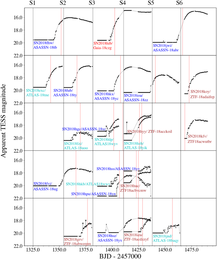
Figure 1. Light curves of the SNe Ia observed in the first six sectors of TESS data. The data were binned to 8 hr and flux-calibrated as described in Section 3. The pre-explosion magnitudes are 3σ upper limits. The SNe are roughly ordered from top to bottom by apparent magnitude at peak. The vertical red lines mark the times of discovery, and the Xs mark outliers caused by asteroids moving through the photometric aperture.
Download figure:
Standard image High-resolution imageTable 1. Properties of the Supernova Sample
| Name | Tpeak | ΔT | MT | νLν | Redshift | E(B − V) | Discovery | Classification | Analysis Notes | ||||||
|---|---|---|---|---|---|---|---|---|---|---|---|---|---|---|---|
| (mag) | (mag) | (mag) a | (erg s−1) | (mag) | Section 4 b | Section 5 c | Flux Cal d | Bkg e | Strap f | Detrend g | |||||
| SN2018exc | ATLAS-18tne | 16.21 | 3.32 | −20.84 ± 0.14 | 3.30 × 1047 | 0.0570 | 0.034 | Tonry et al. (2018e) | Stein et al. (2018) | X | X | ⋯ | ⋯ | ⋯ | ⋯ |
| SN2018fhw | ASASSN-18tb | 16.05 | 3.49 | −18.31 ± 0.43 | 2.96 × 1046 | 0.0170 | 0.027 | Brimacombe et al. (2018b) | Eweis et al. (2018) | X | X | ⋯ | ⋯ | ⋯ | X |
| Kollmeier et al. (2019) | |||||||||||||||
| Vallely et al. (2019) | |||||||||||||||
| SN2018fub | ASASSN-18ty | 16.16 | 3.38 | −19.35 ± 0.26 | 8.07 × 1046 | 0.0288 | 0.011 | Brimacombe et al. (2018c) | Strader (2018) | X | X | ⋯ | ⋯ | ⋯ | ⋯ |
| SN2018fvi | ASASSN-18ug | 17.34 | 2.72 | −20.06 ± 1.14 | 5.54 × 1046 | 0.0404 | 0.025 | Brimacombe et al. (2018d) | Strader (2018) | ⋯ | ⋯ | X | ⋯ | ⋯ | X |
| SN2018fzi | ATLAS-18uoo | 19.18 | 1.22 | −18.70 ± 0.10 | 4.29 × 1046 | 0.0800 | 0.174 | Tonry et al. (2018f) | Fremling et al. (2018a) | ⋯ | ⋯ | ⋯ | ⋯ | ⋯ | ⋯ |
| SN2018grv | ZTF-18abwerpm | 18.51 | 1.98 | −19.00 ± 0.11 | 6.21 × 1046 | 0.0700 | 0.032 | Fremling (2018a) | Fremling et al. (2018e) | ⋯ | ⋯ | ⋯ | ⋯ | ⋯ | ⋯ |
| SN2018hgc | ASASSN-18xr | 17.02 | 1.91 | −19.82 ± 0.15 | 1.28 × 1047 | 0.0520 | 0.026 | Brimacombe et al. (2018e) | Dimitriadis et al. (2018) | ⋯ | ⋯ | ⋯ | ⋯ | X | ⋯ |
| SN2018hib | Gaia-18czg | 14.90 | 4.70 | −19.36 ± 0.45 | 7.85 × 1046 | 0.0163 | 0.019 | Delgado et al. (2018) | Reguitti et al. (2018) | X | X | ⋯ | ⋯ | ⋯ | X |
| SN2018hka | ATLAS-18wwt | ⋯ | ⋯ | ⋯ | ⋯ | 0.0370 | 0.029 | Tonry et al. (2018a) | Fremling et al. (2018b) | ⋯ | ⋯ | ⋯ | ⋯ | ⋯ | ⋯ |
| SN2018hkb | ATLAS-18wwv | 18.20 | 1.90 | −18.30 ± 0.17 | 2.89 × 1046 | 0.0440 | 0.105 | Tonry et al. (2018a) | Berton et al. (2018) | ⋯ | ⋯ | ⋯ | ⋯ | ⋯ | ⋯ |
| SN2018hkx | ASASSN-18yc | 16.32 | 3.75 | −18.88 ± 0.30 | 5.11 × 1046 | 0.0250 | 0.036 | Nicholls et al. (2018) | Jha et al. (2018) | X | X | ⋯ | ⋯ | ⋯ | ⋯ |
| SN2018hlp | ATLAS-18wyv | 18.15 | 1.59 | −19.18 ± 0.12 | 7.37 × 1046 | 0.0650 | 0.021 | Tonry et al. (2018b) | Payne et al. (2018) | ⋯ | ⋯ | ⋯ | ⋯ | ⋯ | ⋯ |
| SN2018hpu | ASASSN-18yn | 18.43 | 3.25 | −18.93 ± 0.32 | 5.94 × 1046 | 0.0660 | 0.013 | Brimacombe et al. (2018a) | Hiramatsu et al. (2018a) | X | ⋯ | ⋯ | ⋯ | X | ⋯ |
| SN2018hss | ASASSN-18yv | 17.10 | 0.59 | −19.30 ± 0.18 | 7.92 × 1046 | 0.0430 | 0.009 | Brimacombe et al. (2018f) | Hiramatsu et al. (2018b) | ⋯ | ⋯ | ⋯ | ⋯ | ⋯ | X |
| SN2018hsz | ASASSN-18yx | 17.55 | 2.38 | −20.52 ± 1.16 | 1.16 × 1047 | 0.0617 | 0.013 | Brimacombe et al. (2018g) | Burke et al. (2018) | ⋯ | ⋯ | X | ⋯ | ⋯ | ⋯ |
| SN2018huc | ZTF-18acbvcmw | 17.92 | 1.63 | −19.68 ± 0.11 | 1.19 × 1047 | 0.0730 | 0.019 | Fremling (2018b) | Fremling et al. (2019b) | ⋯ | ⋯ | ⋯ | ⋯ | ⋯ | ⋯ |
| SN2018hyy | ZTF-18acckoil | 16.53 | 2.79 | −19.00 ± 0.25 | 5.77 × 1046 | 0.0290 | 0.025 | Fremling (2018c) | Fremling et al. (2018c) | ⋯ | ⋯ | ⋯ | ⋯ | ⋯ | ⋯ |
| SN2018hzh | ATLAS-18yik | 16.77 | 3.59 | −19.17 ± 0.21 | 6.99 × 1046 | 0.0350 | 0.005 | Tonry et al. (2018c) | Bose et al. (2018) | X | ⋯ | ⋯ | ⋯ | ⋯ | ⋯ |
| SN2018ieu | ZTF-18acdzzyf | 17.76 | 2.01 | −18.51 ± 0.19 | 3.79 × 1046 | 0.0405 | 0.019 | Nordin et al. (2018a) | Fremling et al. (2018d) | ⋯ | ⋯ | ⋯ | ⋯ | ⋯ | ⋯ |
| SN2018ioa | ASASSN-18zz | 17.59 | 2.72 | −19.38 ± 1.10 | 4.59 × 1046 | 0.0412 | 0.021 | Brimacombe et al. (2018h) | Bose et al. (2018) | ⋯ | ⋯ | X | X | ⋯ | X |
| SN2018jnd | ATLAS-18baqy | 18.81 | 1.16 | −19.30 ± 0.09 | 8.13 × 1046 | 0.0900 | 0.088 | Tonry et al. (2018d) | Fremling et al. (2018f) | ⋯ | ⋯ | ⋯ | ⋯ | X | ⋯ |
| SN2018jwi | ASASSN-18abr | 15.05 | 4.89 | −19.29 ± 0.43 | 7.25 × 1046 | 0.0170 | 0.064 | Cacella et al. (2018) | Pursiainen et al. (2018) | X | ⋯ | X | X | ⋯ | ⋯ |
| SN2018kfv | ZTF-18acwutbr | 17.17 | 2.90 | −16.36 ± 0.66 | 3.72 × 1045 | 0.0110 | 0.299 | Fremling (2018d) | Fremling et al. (2019a) | ⋯ | ⋯ | ⋯ | ⋯ | ⋯ | X |
| SN2018koy | ZTF-18adaifep | 17.09 | 3.44 | −18.65 ± 0.24 | 3.79 × 1046 | 0.0310 | 0.122 | Nordin et al. (2018b) | Pineda et al. (2019) | X | X | ⋯ | ⋯ | ⋯ | ⋯ |
Notes. Absolute magnitudes MT are calculated from the classification redshift and corrected for Galactic extinction using the Cardelli et al. (1989) extinction law with RV = 3.1 and the given value of E(B − V) from Schlafly & Finkbeiner (2011). We assume an error of 1000 km s−1 on the redshifts, due to the difficulty of separating blue-shifted SN emission in the line profile from the hosts cosmological redshift. No K correction is applied. Apparent peak magnitudes Tpeak are observed values, uncorrected for Galactic extinction.
a The absolute magnitude for SN2018kfv is implausibly low for the redshift reported to TNS. The classification spectrum is low-resolution and consistent with redshifts up to 0.03. At z = 0.03, the absolute magnitude of SN2018kfv would be −18.9. b Sources marked with an “X” were fit with a power law to characterize the early light curve, as described in Section 4. They all have Δ T > 3.0 (column 4). c Sources marked with an “X” were searched for signatures of companion stars, as described in Section 5. SN2018hpu, SN2018hzh, and SN2018jwi were not analyzed because of large gaps in the light curves near the times of first light. d Sources marked with an “X” were flux calibrated across two sectors using a joint fit to both data sets, as described in Section 3. e Sources marked with an “X” were near strong scattered light backgrounds at the time of first light, and these times were manually excluded as described in Section 3.1. f Sources marked with an “X” are affected by pixels with enhanced sensitivity from “straps,” as described in Section 3.1. g Sources marked with an “X” were near bright stars and required detrending, as described in Section 3.1.Table 2. TESS SN Light Curves
| Name | BJD-2,457,000.0 | Flux | Asteroid | |
|---|---|---|---|---|
| (days) | (e s−1) | |||
| SN 2018exc | ATLAS-18tne | 1325.325680 | −1.87 ± 2.02 | 0 |
| SN 2018exc | ATLAS-18tne | 1325.346510 | 3.12 ± 2.03 | 0 |
| SN 2018exc | ATLAS-18tne | 1325.367340 | −0.44 ± 2.06 | 0 |
| ⋯ | ⋯ | ⋯ | ⋯ | |
Note. The light curves for all the SNe are presented in a single table. The “Asteroid” column presents a boolean value that marks epochs in which we identified asteroids moving through the photometric apertures.
Only a portion of this table is shown here to demonstrate its form and content. A machine-readable version of the full table is available.
Download table as: DataTypeset image
For six objects (SN 2018fhw, SN 2018fvi, SN 2018hib, SN 2018hkx, SN 2018ioa, and SN 2018jwi), we were also able to measure Δm15 (the decline in the light curve 15 days after peak; Phillips 1993) and thereby estimate the absolute magnitudes independently of the redshifts. To determine Δm15, we used SNooPy (Burns et al. 2011) to fit i-band SN Ia templates to the TESS light curves. The templates were adapted to the TESS instrument response neglecting any internal host-galaxy extinction and using the template Type Ia spectral energy distributions (SEDs) of Hsiao et al. (2007) to calculate K corrections. The differences between the absolute magnitudes determined using the redshift-based distances and those determined using Δm15 ranged from −0.29 to 0.35 mag. The mean difference was 0.03 mag in the sense that the Δm15 distances were slightly larger than the redshift-based distances. The values of Δm15 for SN 2018fhw, SN 2018fvi, SN 2018hib, SN 2018hkx, SN 2018ioa, and SN 2018jwi were 1.80, 0.84, 0.18, 1.68, 0.60, and 1.26 mag, respectively, all with uncertainties of 0.06 mag. Our estimate of Δm15 for SN 2018fhw is 0.2 mag smaller than the estimates in Kollmeier et al. (2019) and Vallely et al. (2019), who used ground-based BVri-band photometry and Swift UV/optical light curves to derive Δm15. This discrepancy is partly due to the fact that the value of Δm15 reported here is for the i band, while Kollmeier et al. (2019) and Vallely et al. (2019) reported Δm15 for the B band. Those studies also used color information to constrain the intrinsic SN spectrum and K corrections, and so we expect their estimates of Δm15(B) to be more accurate. The systematic errors in the redshift-based distances of local SNe primarily arise from the difficulty of separating blueshifted SN emission in the line profile from the host’s cosmological redshift. Since we did not have late-time light curves for all of the SNe and therefore did not have a complete set of Δm15 estimates, we used the redshift-based distances for consistency. Future work may leverage additional multiwavelength observations of these SNe to tightly constrain Δm15 and provide more precise distances.
3.1. TESS Systematic Errors
Even after image subtraction, the TESS FFIs are subject to several systematic errors. We describe each effect and our strategy to mitigate these issues below. Table 3 summarizes the steps that we applied to flag and remove problematic data. Appendix A shows the detailed light curves for each SN and the auxiliary data used to identify and remove problematic epochs.
- 1.Pointing jitter during an exposure increases the observed noise due to flux leaving the photometric aperture and intrapixel variations. Although the difference imaging method helped correct some of these losses, periods of large jitter were imperfectly corrected. We considered time periods with high pointing jitter unreliable and removed them from further analysis. Such time periods were identified by binning the mission-supplied guiding offsets in quaternion form 21 to the 30 minute intervals of each FFI and performing three rounds of 5σ clipping using both the binned quaternions and the standard deviation within each bin. The epochs removed for each light curve using this method are shown in the figures in Appendix A.
- 2.Scattered light from the Earth and Moon is the main source of systematic errors in our light curves and set the limit on the accuracy of our photometry. Scattered light is apparent in the FFIs when the Earth or Moon moves within 37° of a camera boresight. At these times, the image backgrounds become quite high, and strong, rapidly changing glints appear and move through the images. These issues are described in detail in Vanderspek et al. (2018, especially their Figures 7.2, 7.4, and 7.7). Times affected by scattered light were recorded in the data release notes for each sector. Although the local background corrections described in Section 3 accounted for most of these issues, strong gradients and high-frequency spatial features in the scattered-light pattern still caused significant systematic errors for faint sources such as the SN analyzed here. We estimated that the background corrections during these problematic times were typically accurate to about 0.2%–0.6% of the mean background level. However, larger deviations were observed, and even ∼0.1% errors in the background corrections are significant for faint SN light curves. For time periods with enhanced background levels or strong scattered-light signals, we did not consider the photometry reliable and removed such data from further analysis. We identified these time periods using three rounds of 5σ clipping on the local background estimates. This procedure removed outliers in the distribution of background estimates and caught most rapidly moving glints. All epochs removed by sigma clipping of the backgrounds are shown in Appendix A.Sigma clipping did not perform very well when the Earth or Moon rose above or set below the spacecraft sunshade. We therefore flagged additional images based on visual inspection of the difference images. The problem was most acute at the ends of Sector 4 and Sector 5, for which we manually excluded data from the light curves of SN 2018ioa (Sector 4, BJD-2,457,000 = 1436.020 to 1436.812) and SN 2018jwi (Sector 5, BJD-2,457,000 = 1463.605 to 1464.251). The TESS mission also excluded these time intervals from their transiting-planet searches because of strong and rapidly changing background features. SN 2018ioa and SN 2018jwi were the only sources for which these features occurred during the early-time light curves—other sources were clearly affected at these times, but the scattered light did not affect the initial rise and so the data are shown in Figure 1 for completeness. We also found some evidence of residual background errors in the light curves from Sectors 1 and 2 of SN 2018exc, SN 2018fhw, and SN 2018fub based on visual inspection. In these cases, there was no clear justification for excluding the data, but it was likely that the early-time light curves were affected. We therefore included the data in further analysis but regarded the results with caution (see Section 4 below).
- 3.Metallic “straps” at the bottom of the CCDs reflect long-wavelength photons and result in heightened pixel sensitivity for certain columns in the imaging array (Vanderspek et al. 2018; Section 6.6.1). Although the straps did not affect differential photometry of the SN flux, they did affect the local background during periods of strong scattered light. We found that it was possible to correct for the effects of the straps using a technique similar to illumination corrections developed for long-slit spectroscopy. We median-filtered the difference images along each affected column to make a smooth estimate of the enhanced background, subtracted the result from the column in question, and interpolated the local background along the rows. Although the correction was not perfect, in most cases it greatly improved the photometry. Only SN 2018hgc, SN 2018hpu, and SN 2018jnd were near enough to CCD straps to be affected by this procedure.
- 4.In some cases, bright (T < 18) asteroids move through the photometric aperture and cause a small bump in the light curve over several hours. The simplest way to identify these cases was inspection of the difference images. Given the short period of time over which such events occurred, we flagged and ignored the affected parts of the light curve. The probability of an asteroid passing through the photometric aperture is highest for transients in Camera 1, which was pointing nearest the ecliptic plane. SN 2018grv, SN 2018hgc, SN 2018hka, SN 2018hkb, and SN 2018hyy all suffered from this effect. The epochs affected by asteroids are flagged in the light curves given in Table 2 and explicitly highlighted in the figures in Appendix A.
- 5.The final class of systematic errors is for SNe that occurred near a bright star in the TESS images. Imperfect residuals in the difference images can then contaminate the photometric aperture. Given the large plate scale (2119 per pixel), this was a common effect: SN 2018fhw, SN 2018fvi, SN 2018hib, SN 2018hss, SN 2018ioa, and SN 2018kfv were all affected. For all of these sources, there was a very bright star within 2 or 3 pixels with obvious residuals in the difference images. We were able to remove the main effects of these residuals by (1) extracting the light curves of the contaminating stars, (2) smoothing with a median filter, and (3) fitting a shift and scale factor to the affected parts of the SN light curves. We then subtracted the scaled and smoothed star’s light curve from the SN light curve. The light curves of the contaminating star, the smoothed model, the fit to the SN light curve, and the corrected SN light curve are shown in Appendix B for all affected sources. For SN 2018fhw, we found better results using FFIs without Gaussian smoothing in the image subtraction (see Section 3). A detailed discussion of detrending for SN 2018fhw is given by Vallely et al. (2019; see their Figures 3 and 5). For SN 2018hss, a bright star was extremely close to the SN in the image, and we were not able to improve the light curve using this method. We present our differential measurements in Appendix A for completeness, but we do not regard the light curve as reliable. A more sophisticated detrending algorithm might help with this problem in the future.
Table 3. Systematic Errors in TESS SN Light Curves
| Issue | Solution | Number of Affected SNe |
|---|---|---|
| Pointing jitter | Three rounds of 5σ clipping on | |
| (a) 30 minute binned guiding offset quaternions and | ||
| (b) standard deviations of quaternions within each bin | 24 | |
| Scattered light/glints | Three rounds of 5σ clipping on the local background estimates | 24 |
| Removed 0.8 days of data at the ends of Sector 4 and Sector 5 | 2 | |
| Enhanced background | ||
| from “straps” | Median-filtered image columns and interpolated along rows | 3 |
| Asteroids | Visual inspection of difference images | 5 |
| Blended bright star | Fit a scaled version of the starlight curve | 6 |
Note. Summary of systematic errors in TESS SN light curves and steps taken to flag/remove problematic data. A detailed discussion is given in Section 3.1. Appendix A shows the full SN light curves and the time series of the binned quaternions, the standard deviations within each bin, and the local background estimates used for sigma clipping.
Download table as: ASCIITypeset image
4. Analysis
For light curves with sufficient dynamic range between the initial detection and the peak, it is possible to gain insight into the explosion physics and place limits on the size of any companions. We began by parameterizing the light curves with a rising power-law fit of the form

where t0 is the time of the first detection; A, B, and β are constants; and H(t) is the Heaviside function. The parameter B accounts for any residual background flux at early times and must be included to properly estimate uncertainties in β. We constrained β between 0.5 and 4.0, and we required that A be greater than 0. Following Olling et al. (2015), we only fit the light curves up to 40% of the peak flux. We estimated the uncertainties on the fitted parameters with 1000 iterations of bootstrap resampling of the light curves and report the widths of the central 68% confidence intervals of the resulting parameter distributions.
We focused on the nine SNe with ΔT > 3.0 mag, namely, SN 2018exc, SN 2018fhw, SN 2018fub, SN 2018hib, SN 2018hkx, SN 2018hpu, SN 2018hzh, SN 2018jwi, and SN 2018koy. For SN 2018hzh, the onset of the light-curve rise was missing due to data gaps. A large portion of the early rise of SN 2018jwi was also missing, although we detected the onset of its rise. For these cases, our fitting procedure was still able to constrain t0 and β if we extrapolated the observed power law through the gaps. However, we must fit SN 2018jwi up to 60% of the peak flux to meaningfully constrain the power-law index after the gap. We also fit SN 2018fhw up to 60% of the peak flux, because the data were affected by scattered light at the time that the light curve reached 40% of the peak flux. There was a visual change in the curvature of the light curve at this time, which was related to the Earth setting below the TESS sunshade at BJD-2,457,000 ∼ 1350.4. Fitting over the longer baseline averaged over any errors in the background subtraction and should lead to a more robust result. A detailed view of this part of the SN 2018fhw light curve is shown in Figure 2.
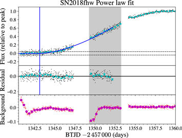
Figure 2. Power-law fit, residuals, and local background estimates for SN 2018fhw near the time of first light. The small points are the individual 30 minute FFI exposures, and the larger circles are averages over 8 hr. All units are flux relative to peak. The vertical blue line is the fitted time of first light, while the solid blue line shows the best-fit power-law model. The Earth set below the spacecraft sunshade at BJD-2,457,000 ∼ 1350.4 days, which was responsible for the sudden change in the local background at this time. The gray shaded region highlights times over which there is a visual change in curvature in the light curve, discussed in Section 4. See Appendix A for the full light curve.
Download figure:
Standard image High-resolution imageTable 4 gives the best-fit values of t0 and β from the rising power-law fits. For reference, a fiducial “fireball” model with a constant-temperature photosphere expanding at a constant velocity (Riess et al. 1999) has a rising power-law index of β = 2.0 at wavelengths on the Rayleigh–Jeans tail of the SED. Five of the nine SNe had β > 1.6, and all but one of these (SN 2018exc) were consistent with the fireball model at or very near the 3σ level. The best-fit index for two sources was higher than β = 3.0 (SN 2018exc and SN 2018fub). Of the remaining four SNe, three had indices β ≈ 1.0 (SN 2018hkx, SN 2018hpu, and SN 2018koy), although SN 2018hpu was consistent with 2.0 at the 3σ level. Finally, the index for SN 2018hzh was too uncertain for us to conclude that it was either low or high (β = 0.58 ± 0.83).
Table 4. Power-law Fit Parameters
| Name | t0 | β | dof | χ2/dof | Comments a | |
|---|---|---|---|---|---|---|
| (BJD-2,457,000) | ||||||
| SN 2018exc | ATLAS-18tne | 1329.09 ± 1.26 | 4.00 ± 0.41 | 754 | 0.83 ± 0.05 | Complicated background |
| SN 2018fhw | ASASSN-18tb | 1343.12 ± 0.84 | 1.63 ± 0.33 | 984 | 1.34 ± 0.05 | Complicated background; fit up to 60% of peak |
| SN 2018fub | ASASSN-18ty | 1356.13 ± 1.11 | 3.67 ± 0.55 | 530 | 1.19 ± 0.06 | Complicated background |
| SN 2018hib | Gaia-18czg | 1395.70 ± 0.36 | 2.40 ± 0.12 | 734 | 1.22 ± 0.05 | |
| SN 2018hkx | ASASSN-18yc | 1400.66 ± 0.19 | 1.26 ± 0.09 | 725 | 0.90 ± 0.05 | |
| SN 2018hpu | ASASSN-18yn | 1401.28 ± 0.87 | 1.00 ± 0.39 | 721 | 1.55 ± 0.05 | |
| SN 2018hzh | ATLAS-18yik | 1423.88 ± 2.11 | 0.58 ± 0.83 | 406 | 1.04 ± 0.07 | Gaps near first light |
| SN 2018jwi | ASASSN-18abr | 1459.07 ± 1.17 | 2.85 ± 0.57 | 325 | 1.55 ± 0.08 | Gaps near first light; fit up to 60% of peak |
| SN 2018koy | ZTF-18adaifep | 1470.32 ± 0.35 | 1.28 ± 0.14 | 359 | 1.12 ± 0.07 | |
Note. Uncertainties are central 68% confidence intervals for fits to 1000 iterations of bootstrap resampling.
a This column lists various issues associated with each SN light curve and the resulting fits. Details are discussed in Section 4.Download table as: ASCIITypeset image
We did not find any correlation between the power-law indices and Tpeak or ΔT, so we do not attribute these results to observational effects, such as the signal-to-noise ratio or our fitting procedure. However, there are reasons to be cautious in regard to three of the fits. The light curves for the SNe with power-law indices β > 3.0, SN 2018exc and SN 2018fub, were obtained from images with a complicated background that may have affected the light curve (see Section 3.1). A similar concern exists for SN 2018fhw, although our fits for t0 and β are in good agreement with those reported by Vallely et al. (2019; t0 = 1341.68 ± 0.16 in our units and β = 1.69 ± 0.04). 22 Meanwhile, the light curve of the SN with the lowest power-law index, SN 2018hzh, had a large gap around the onset of the rise in flux. For this SN, t0 was determined by extrapolating from the power-law slope observed at significantly later times, which may not reflect the properties of the rise at the time of explosion.
The values of χ2 per degree of freedom (χ2/dof) were consistent with unity for all sources except SN 2018fhw, SN 2018hpu, and SN 2018jwi. For SN 2018fhw and SN 2018hpu, the discrepancy resulted from outliers in the pre-explosion light curves, which were caused by errors in the local background corrections (see Appendix A). For SN 2018jwi, the issue was probably related to the gap between Sectors 5 and 6 during the early part of the light curve’s rise and to the difficulty of simultaneously fitting the power-law index and the calibration offset for the second sector of data.
In an analysis of a large sample of ground-based early-time SN Ia light curves, Firth et al. (2015) found a range of rising power-law indices, with a mean value of β = 2.44 ± 0.13. In a study of 127 SNe Ia using ZTF data, Miller et al. (2020b) found an average rising power-law index of ∼2 in the r band with an rms scatter of 0.5 and considerable diversity among the SNe. Our findings are consistent with both of these results (although see Miller et al. 2020b Section 9.2 for a discussion of bias in the estimate of the power-law index from Firth et al. 2015). We found three objects out of nine with a power-law index significantly less than 2: SN 2018hkx, SN 2018hpu, and SN 2018koy. Departures from a simple fireball model have been seen in other objects—for example, in SN 2013dy, SN 2014J, SN 2012fr, iPTF 16abc, and ASASSN-18bt (Zheng et al. 2013, 2014; Goobar et al. 2015; Siverd et al. 2015; Contreras et al. 2018; Miller et al. 2018; Shappee et al. 2019, respectively). These sources exhibited more nearly linear rises in the optical for a few days, followed by sharper rises with power-law indices closer to 2. Contreras et al. (2018) showed that the light curve of SN 2012fr is consistent with a moderately mixed initial nickel profile, as modeled by Piro & Morozova (2016). Shappee et al. (2019) found that the early light curve of ASASSN-18bt is also broadly consistent with the models of Piro & Morozova (2016), although Magee & Maguire (2020) argue that the color and spectral evolution of the transient are not consistent with an inhomogeneous 56Ni distribution. In our sample, the light curves of SN 2018hkx and SN 2018hpu could be consistent with this picture, although there was a 4 day gap in observations at the end of Sector 3 for both sources when the nonlinear phase would be expected to begin. On the other hand, the behavior of SN 2018koy is difficult to reconcile with the Piro & Morozova (2016) models. There is no strong evidence for an increase in the slope during the rise of this source; if anything, the slope may be diminishing 7 to 10 days post-explosion.
Interactions between the expanding SN ejecta and a companion star also affect the observed behavior of early-time SN Ia light curves. Based on its blue color at early times, Dimitriadis et al. (2019) interpret the double power law in ASASSN-18bt as the result of a flux excess from a companion interaction superimposed on a fireball light curve. We investigate the effects of companion stars on the TESS light curves in Section 5, to determine if such models can account for the behavior observed in SN 2018hkx, SN 2018hpu, and SN 2018koy described above. We also discuss the interpretation of SNe Ia with blue flux excesses in Section 5.3 (SN 2012cg, iPTF 14atg, SN 2017cbv, HSC 17bmhk, and SN 2019yvq).
Figure 3 shows the power-law indices as a function of peak SN absolute magnitude, with the sources requiring interpolation near t0 represented by open circles. The SNe with lower power-law indices had absolute magnitudes fainter than −19, putting them on the fainter end of the distribution of Type Ia luminosities. For comparison, the results for the Kepler SNe (Olling et al. 2015; Shappee et al. 2019) are shown in blue and cyan, corrected from the Kepler to the TESS bandpass based on the Hsiao et al. (2007) template SED.
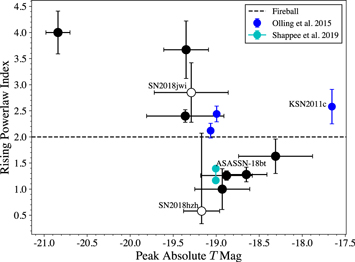
Figure 3. Rising power-law index β as a function of absolute magnitude for the nine SNe observed by TESS with ΔT > 3.0 mag (black points). Objects that required extrapolation to t0 are shown with open circles. For comparison, results from Kepler (Olling et al. 2015; Shappee et al. 2019) are also shown (including both power-law indices of the double-component fit for ASASSN-18bt).
Download figure:
Standard image High-resolution image5. Comparison to Companion Models
Next, we compare the TESS light curves to analytic models from Kasen (2010) that describe the interaction of the SN ejecta with a companion star. In these models, the ejected material from the SN forms a bow shock as it encounters the companion star, producing a flash of X-ray emission followed by a quick rise and then a slow decay of thermal emission at UV/optical wavelengths. The observed light curve depends on the viewing angle of the observer because the viewing angle determines the solid angle of the shocked ejecta on the sky. A viewing angle of 0° places the companion in front of the SN explosion and maximizes the visibility of the shocked material, while a viewing angle of 180° places the companion behind the exploded star so that no emission from the shocked material can be observed. The other parameters of the Kasen (2010) model are the separation of the white dwarf and secondary companion star (which sets the Roche lobe radius of the secondary) and the mass, velocity, and opacity of the SN ejecta. In all calculations that follow, we adopt the fiducial model of Kasen (2010), with a viewing angle of 45°, an ejecta mass of 1.4 M⊙, a velocity of 104 km s−1, and an opacity of 0.2 cm2 g−1, while treating the companion separation/radius as a free parameter. The Kasen (2010) models assume that the companion fills its Roche lobe, and so the companion separation can be used to estimate its radius. The conversion between companion separation and radius depends weakly on the mass ratio of the white dwarf to the companion star, and we assume masses of 1.4 M⊙ and 1.0 M⊙, respectively. This choice is unimportant at the level of detail presented here.
Maeda et al. (2018) derived light-curve models similar to those of Kasen (2010) for different assumptions about how energy from the SN explosion is thermalized when colliding with the companion star. In contrast, Kutsuna & Shigeyama (2015) used simulations to argue that the Kasen (2010) models overpredict the companion signature, although their simulations did not include opacity from free–free emission and Compton scattering and so may have underestimated the luminosity of the shocked region. More theoretical work might lead to a better understanding of the details of the companion signature models and how to best distinguish companion signatures from other effects, such as interactions with CSM and inhomogeneities in the distribution of 56Ni in the SN ejecta (Piro & Morozova 2016; Contreras et al. 2018; Maeda et al. 2018; Magee et al. 2020; Magee & Maguire 2020). For now, we use the Kasen (2010) models, since they provide simple analytic prescriptions for the calculation of light curves and can easily be compared with observational studies that use the same models (e.g., Cao et al. 2015; Hosseinzadeh et al. 2017; Shappee et al. 2019; Miller et al. 2020a).
We calculated the light curves of these companion interaction models using synthetic photometry to combine the TESS wavelength-dependent response function, a blackbody spectrum with the temperature and photospheric radius defined by Equations (24) and (25) of Kasen (2010), and the appropriate luminosity distance for each source (based on the redshifts in Table 1). Our calculations incorporated the effects of redshift on the rest-frame SED and time dilation on the light curves, although these effects were very small. We did not include the effects of the travel time of the SN ejecta to the companion, because the Kasen (2010) models assume that the shocked ejecta expand homologously and are not valid at early times before a self-similar state is reached. The ejecta travel timescale is less than 15 minutes for the majority of the models we employ and so is shorter than the TESS FFI cadence. However, the ejecta travel timescale could reach up to 3–12 hr for the largest separations that we considered (>1013 cm). For convenience, we provide the TESS light-curve models at a fiducial distance of 100 Mpc in Table 5 and note that the flux can be rescaled with reasonable accuracy based on the luminosity distance alone.
Table 5. TESS Light Curves for Kasen (2010) Models at 100 Mpc a
| Time | 50 R⊙ | 25 R⊙ | 10 R⊙ | 5.0 R⊙ | 1.0 R⊙ | 0.5 R⊙ | 0.1 R⊙ | |||||||
|---|---|---|---|---|---|---|---|---|---|---|---|---|---|---|
| (days) | (e s−1) | (mag) | (e s−1) | (mag) | (e s−1) | (mag) | (e s−1) | (mag) | (e s−1) | (mag) | (e s−1) | (mag) | (e s−1) | (mag) |
| 0.001023 | 0.006878 | 25.8464 | 0.005772 | 26.0367 | 0.004573 | 26.2895 | 0.003825 | 26.4835 | 0.002537 | 26.9293 | 0.002121 | 27.1239 | 0.001392 | 27.5807 |
| 0.022525 | 0.164560 | 22.3992 | 0.136899 | 22.5990 | 0.106924 | 22.8673 | 0.088239 | 23.0758 | 0.056138 | 23.5669 | 0.045806 | 23.7877 | 0.027846 | 24.3281 |
| 0.044027 | 0.322945 | 21.6672 | 0.267421 | 21.8720 | 0.207291 | 22.1485 | 0.169844 | 22.3649 | 0.105653 | 22.8803 | 0.085075 | 23.1155 | 0.049556 | 23.7023 |
| ⋯ | ⋯ | ⋯ | ⋯ | ⋯ | ⋯ | ⋯ | ⋯ | ⋯ | ⋯ | ⋯ | ⋯ | ⋯ | ⋯ | ⋯ |
Note.
a In the local universe, the effects of time dilation and K corrections are negligible, and these light curves can be rescaled based on luminosity distance alone.Only a portion of this table is shown here to demonstrate its form and content. A machine-readable version of the full table is available.
Download table as: DataTypeset image
We investigated two issues relating to the signatures of companions in SN Ia light curves. First, we quantified the effect that the presence of a companion signature would have on the observed shape of the light curves. Second, we placed limits on the maximum companion signature detectable in the TESS light curves.
5.1. Effect of Companions on Light-curve Shape
To begin, we simulated SN light curves and investigated the effect that a range of Kasen (2010) models would have on a single power-law fit. We simulated companion interaction models over a range of companion radii from 1 R⊙ to 200 R⊙. Light curves were calculated by adding the Kasen (2010) companion model light curves to a fireball t2 rise. The observed flux in the TESS band of the fireball was calculated using synthetic photometry on a 104 K blackbody spectrum, assuming a sphere with an initial radius of 3 × 108 cm expanding at 109 cm s−1. To convert to flux, we arbitrarily placed the source at z = 0.01 (43 Mpc). We also experimented with the models of Piro (2012), which predict the temperature and photospheric radius of a hot shell of SN ejecta powered by the radioactive decay of 56Ni. However, the normalizations of the Piro (2012) models only slightly deviate from the t2 fireball model used here, and the dependence of photospheric temperature on time in the Piro (2012) models is very weak. We therefore did not find any important differences when using the Piro (2012) models as compared to using a fireball. The Kasen (2010) companion light-curve models are shown in the left-hand side of Figure 4, while the companion models, the fireball rise, and their sum are shown in the right panels. Finally, we fit these model light curves using Equation (1) described in Section 4 and compared the resulting normalization and power-law indices to the input values. The results are given in Table 6, and the fits and residuals are shown in Figure 5.
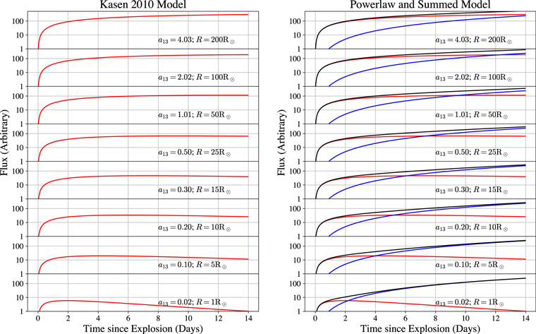
Figure 4. Simulated light curves of the Kasen (2010) companion models used to investigate the signatures of companion stars in our fits from Section 4. The left panel shows the Kasen (2010) models alone (red lines). The parameter a13 is the separation between the exploded star and its companion, in units of 1013 cm; R is the equivalent Roche lobe radius of the companion for a 1.4/1.0 M⊙ primary/secondary system. The right panel shows the same models (red lines), a fireball t2 component for the SN ejecta (blue lines), and the total light curve (black lines).
Download figure:
Standard image High-resolution image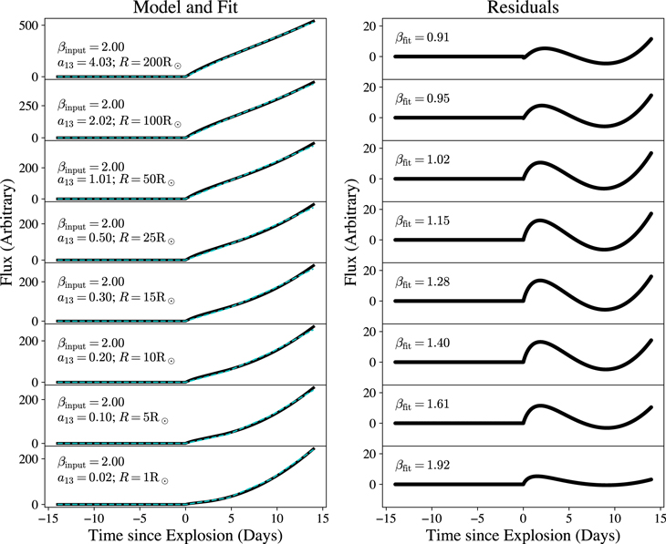
Figure 5. Results for fits of Equation (1) to the simulated light curves from Figure 4. The simulated light curves are shown as black lines in the left panel, and the best-fit power laws are shown as cyan lines. The right panel shows the residuals from the fits. Larger companion radii tended to bias the recovered power-law index β to low values and produced a characteristic pattern of residuals. See Table 6 for details.
Download figure:
Standard image High-resolution imageTable 6. Results for Fits to Simulated Light Curves
| Separation | Radius | t0 | β | Flux at t = 1 day | Background |
|---|---|---|---|---|---|
| (cm) | (R⊙) | (days) | (e s−1) | (e s−1) | |
| Fits without noise | |||||
| 4.03 × 10¹³ | 200 | −0.008 | 0.91 | 47.66 | 0.41 |
| 2.02 × 10¹³ | 100 | −0.008 | 0.95 | 34.48 | 0.71 |
| 1.01 × 10¹³ | 50 | −0.008 | 1.02 | 23.17 | 1.06 |
| 0.50 × 10¹³ | 25 | −0.008 | 1.15 | 14.11 | 1.43 |
| 0.30 × 10¹³ | 15 | −0.008 | 1.28 | 9.18 | 1.65 |
| 0.20 × 10¹³ | 10 | −0.008 | 1.40 | 6.33 | 1.75 |
| 0.10 × 10¹³ | 5 | −0.008 | 1.61 | 3.48 | 1.69 |
| 0.02 × 10¹³ | 1 | −0.008 | 1.92 | 1.52 | 0.84 |
| Fits with noise | |||||
| 4.03 × 10¹³ | 200 | −0.008 | 0.92 | 46.62 | 0.35 |
| 2.02 × 10¹³ | 100 | −0.008 | 0.94 | 35.02 | 0.37 |
| 1.01 × 10¹³ | 50 | −0.008 | 1.02 | 23.15 | 1.13 |
| 0.50 × 10¹³ | 25 | −0.008 | 1.15 | 14.10 | 1.41 |
| 0.30 × 10¹³ | 15 | −0.008 | 1.29 | 8.99 | 1.90 |
| 0.20 × 10¹³ | 10 | −0.008 | 1.40 | 6.32 | 1.51 |
| 0.10 × 10¹³ | 5 | −0.008 | 1.65 | 3.17 | 1.72 |
| 0.02 × 10¹³ | 1 | −0.008 | 1.93 | 1.44 | 1.38 |
Note. Recovered parameters from fits to simulated models of a β = 2 power-law rise (fireball) plus a Kasen (2010) companion model. Larger companions flattened the observed power-law index. The light curves, fits, and residuals are shown in Figures 5 and 6. The parameters of the Kasen (2010) models match the fiducial model described in Section 5.1.
Download table as: ASCIITypeset image
The parameter A in Equation (1) can be interpreted as the flux of the model 1 day after the explosion (t − t0 = 1 day). Larger companions result in larger fluxes after 1 day owing to the significant contribution of flux from the companion component. There is also a small bias in the inferred explosion time t0 to earlier times (−0.008 days, about 11 minutes), although the bias is smaller than the 30 minute TESS FFI cadence. The shapes of the companion light curves have a characteristic t1/2 power law, which leads to a more linear light curve when combined with the intrinsic β = 2 rise. Table 6 shows that the fitted power-law index ranges from 1.76 to 1.9 for small companions with radii ≲ 15 R⊙. This range of companion radii will generally yield results consistent with a fireball model. Larger companion radii (25 R⊙–200 R⊙) result in much lower power-law indices, with β = 1.4–1.1. This result may be consistent with the SNe in this study that show power-law indices close to unity (SN 2018hkx, SN 2018hpu, and SN 2018koy).
However the residuals of these fits show a characteristic pattern where the linear rise underpredicts the companion flux at early times and overpredicts the fireball flux at late times (Figure 5). Thus, it is still possible to distinguish between an intrinsically linear rise in the SN light curve and a large companion.
To compare these simulations to observations, we next refit the models after adding noise. We added Gaussian deviates to each point with a standard deviation equal to 4% of the fireball rise after 14 days, which approximately reproduced our best light curves. These results are shown in Figure 6. Measurement noise washes out most of the residual pattern on 30 minute timescales, but is often recoverable after binning to 8 hr (cyan points in the right panels of Figure 6).
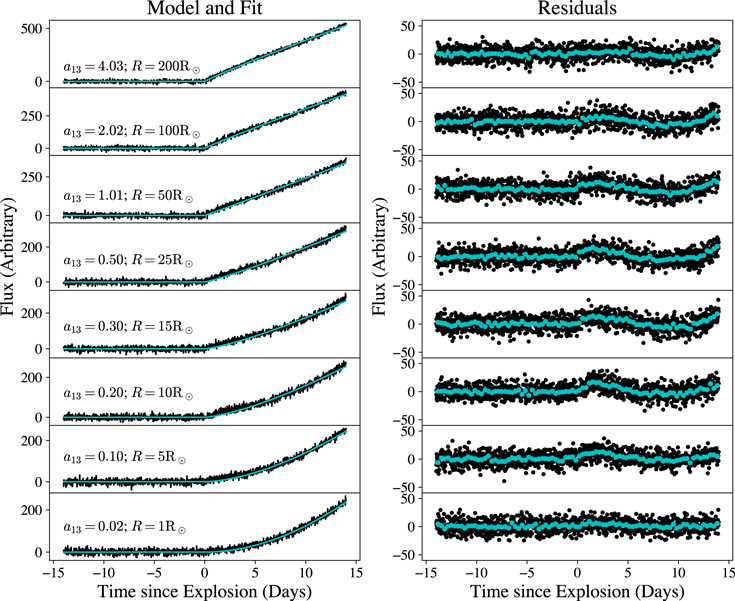
Figure 6. Same as Figure 5, but with random measurement noise added. The cyan circles show the residuals binned to 8 hr. The amplitude of the noise was set to 4% of the flux of the fireball component after 14 days, which is comparable to the observed scatter of our best light curves. Measurement noise washed out much of the pattern in the residuals from Figure 5, but the pattern was still detectable on 8 hr timescales.
Download figure:
Standard image High-resolution imageWe are left with two main conclusions. First, small companions lead to small biases in the power-law index and small systematic residuals. For large companion stars, the power-law rises are very flat, and the residuals show a characteristic pattern associated with the change in power-law index from times when the companion emission dominates to times when the fireball dominates. The detailed residuals can distinguish between an intrinsically linear light curve and a composite fireball-plus-companion light curve, given sufficiently high signal-to-noise ratios.
5.2. Search for Companions in the TESS SN Light Curves
Finally, we searched each SN light curve for companion signatures that match the Kasen 2010 models. We searched a grid of companion models with 20 separations/radii over 70 initial explosion times t0 from −2 to +5 days relative to the value of t0 found in Section 4. For each combination of companion radius and t0, we first subtracted the Kasen (2010) model from the observed light curve and then fit a power-law model, optimizing A, β, and B in Equation (1) (with t0 held fixed) to minimize χ2. The companion separations/radii were equally spaced in logarithm and ranged from 2.2 × 1011 cm to 4 × 1013 cm (1.1 R⊙–223 R⊙), while the values of t0 were evenly spaced every 2.4 hr. We verified that this fitting procedure and grid spacing accurately recovered the parameters of any companion signatures by performing Monte Carlo simulations, the details of which are discussed in Appendix C. We also used these simulations to identify the χ2 values that correspond to the 98% and 99.9% confidence limits on the presence of any companion signatures.
We restricted our analysis to the six SNe where continuous observations were available through a significant portion of the rising light curve (SN 2018exc, SN 2018fhw, SN 2018fub, SN 2018hib, SN 2018hkx, and SN 2018koy). This removed SN 2018hzh, SN 2018hpu, and SN 2018jwi from further consideration. Figure 7 shows the χ2 contours for the six SNe on the grid of companion radii and t0, and Figure 8 shows the best-fit companion and power-law models.
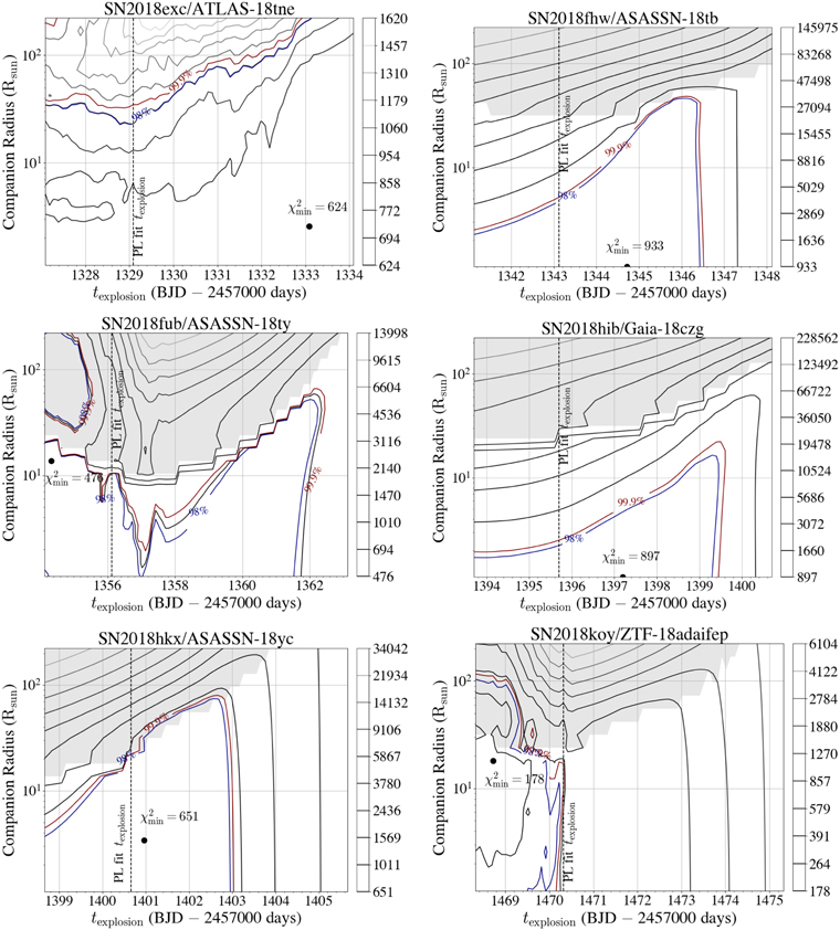
Figure 7. χ2 contours for the grid search of Kasen (2010) companion models discussed in Section 5.2. The minimum value of χ2 is marked for each SN. The gray contours show values of χ2 equally spaced in logarithm, while the gray shaded regions correspond to the nonphysical solutions described in Section 5.2. The blue and red contours mark the 98% and 99.9% confidence intervals of χ2 based on Monte Carlo simulations (see Appendix C). The vertical black dashed lines show the time of explosion derived from the simple power-law fits in Section 4 (see Table 4). The simulations suggest that a strong prior on t0 to match the power-law fits provides a more realistic constraint than the formally allowed maximum radius at the 99.9% confidence interval.
Download figure:
Standard image High-resolution image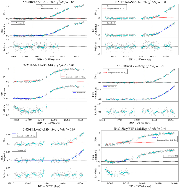
Figure 8. Best-fit companion and power-law models from the grid search in Section 5.2. The top panels show the raw light curve (black dots) and data binned to 8 hr (cyan circles), with the best-fit companion model from Kasen (2010) in red. The middle panels show the data with the Kasen (2010) model subtracted out and the best-fit power law (with t0 held fixed). The bottom panel shows the residuals of the total fit.
Download figure:
Standard image High-resolution imageThe gray regions in Figure 7 show unphysical solutions where subtracting a large companion model caused the light-curve flux to become negative. However, a formally reasonable fit was achieved by forcing the model normalization A to a very small value. In these cases, we flagged solutions where A < 10−7 (in flux units relative to peak) as unphysical. A similar example of this family of solutions is shown in the bottom left panel of Figure 9 for SN 2018hkx; in this case, the normalization is A ≈ 1.8 × 10⁻⁵. We tried refitting the data with a prior on the normalization A of 1/A (such that small A increases χ2), but the simulations showed that this biased the recovered companion separation/radius to the smallest value on the grid in order to keep A as large as possible, even when large companion signatures (>5 R⊙) were injected into the light curves. Thus, in Figure 7 we simply mark unphysical solutions with small values of A. In cases where the 3σ contours extended into nonphysical regions of parameter space, we adopted the solution at fixed t0 with the maximum companion separation/radius and A > 10−7 instead of the 3σ contour. This issue only affected the companion limits for SN 2018hkx and SN 2018koy.
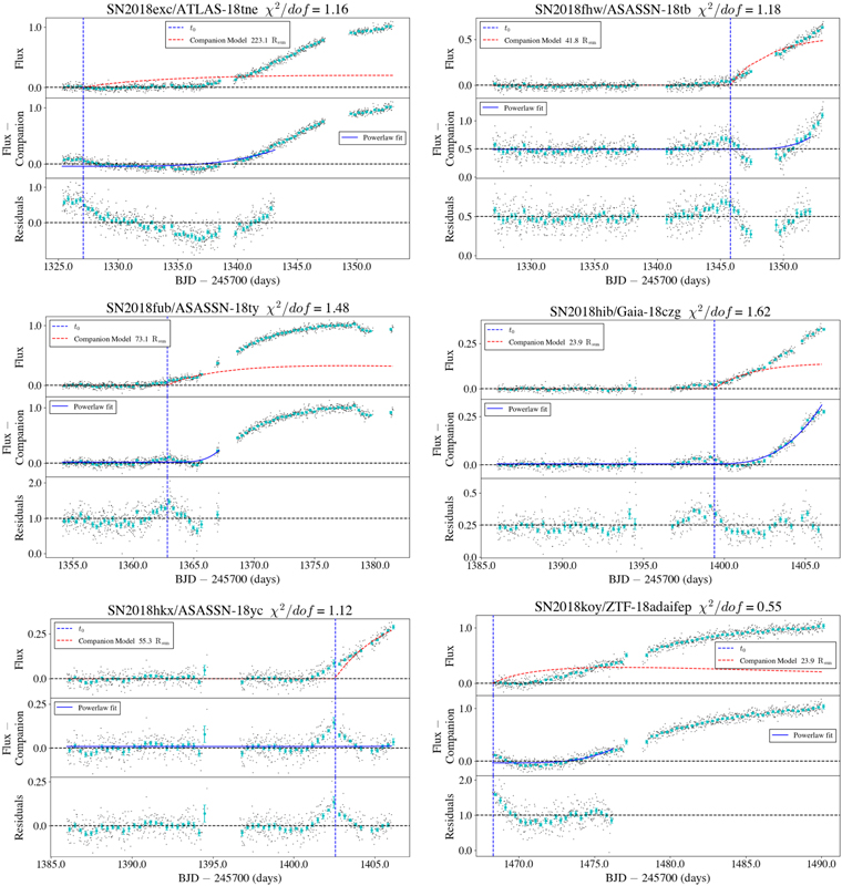
Figure 9. Same as Figure 8, but for the maximum allowable Kasen (2010) model at the 99.9% confidence level (3σ limit).
Download figure:
Standard image High-resolution image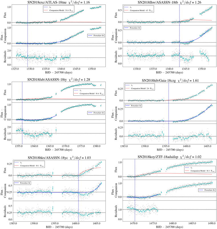
Figure 10. Same as Figure 8, but for the maximum allowable Kasen (2010) model at the 99.9% confidence level (3σ limit) with t0 held fixed to the value in Table 4. Simulations showed that t0 was not significantly biased when fitting a power-law model, while the models in Figure 9 push t0 to significantly later times. We therefore adopted these models as our final 3σ limits.
Download figure:
Standard image High-resolution imageFor each SN, there are three solutions of particular interest: the best fit, the 3σ limit for the maximum companion separation/radius, and the 3σ limit at the time of explosion inferred from the initial fit in Section 4. The parameters for these solutions are shown in Table 7, where the uncertainties on A and β are from the formal errors in the fits. Figures 8–10 show each of these solutions for each SN. For simplicity, we only discuss the results in terms of the companion model radii, although this is equivalent to using the companion separation because the Kasen (2010) models assume Roche lobe overflow. The best-fit companion radii of SN 2018exc, SN 2018fhw, SN 2018hib, and SN 2018hkx are all less than 4 R⊙. The best-fit radii for SN 2018fhw and SN 2018hib are the minimum value for the search of 1.1 R⊙. SN 2018fub and SN 2018koy had larger best-fit values of 13.7 R⊙ and 18.1 R⊙, respectively. However, these models overpredict the flux at early times and are unlikely to be physical even if they formally have the best χ2 (see Figure 8).
Table 7. Upper Limits on Companion Parameters for Kasen (2010) Models
| Name | Separation | Radius | t0 | β | A | dof | χ2/dof | |
|---|---|---|---|---|---|---|---|---|
| (1013 cm) | (R⊙) | (BJD-2,457,000) | ||||||
| Best Fit | ||||||||
| SN 2018exc | ATLAS-18tne | 0.05 | 2.6 | 1333.09 | 2.74 ± 0.09 | 7.32e-04 ± 1.42e-04 | 755 | 0.83 ± 0.05 |
| SN 2018fhw | ASASSN-18tb | 0.02 | 1.1 | 1344.72 | 1.37 ± 0.03 | 3.53e-02 ± 2.18e-03 | 947 | 0.99 ± 0.05 |
| SN 2018fub | ASASSN-18ty | 0.25 | 13.7 | 1354.33 | 4.00 ± 0.00 | 1.16e-05 ± 6.56e-06 | 531 | 0.90 ± 0.06 |
| SN 2018hib | Gaia-18czg | 0.02 | 1.1 | 1397.20 | 2.10 ± 0.02 | 3.55e-03 ± 1.77e-04 | 735 | 1.22 ± 0.05 |
| SN 2018hkx | ASASSN-18yc | 0.06 | 3.4 | 1400.96 | 1.65 ± 0.08 | 1.66e-02 ± 1.98e-03 | 726 | 0.90 ± 0.05 |
| SN 2018koy | ZTF-18adaifep | 0.33 | 18.1 | 1468.72 | 3.85 ± 0.44 | 1.20e-04 ± 1.05e-04 | 360 | 0.50 ± 0.07 |
| Max Companion (3σ limit) | ||||||||
| SN 2018exc | ATLAS-18tne | 4.02 | 223.1 | 1327.09 | 4.00 ± 0.33 | 4.35e-06 ± 3.87e-06 | 755 | 1.17 ± 0.05 |
| SN 2018fhw | ASASSN-18tb | 0.75 | 41.8 | 1345.82 | 4.00 ± 1.18 | 6.60e-05 ± 1.36e-04 | 947 | 1.18 ± 0.05 |
| SN 2018fub | ASASSN-18ty | 1.32 | 73.1 | 1362.83 | 4.00 ± 1.25 | 6.41e-04 ± 9.45e-04 | 531 | 1.49 ± 0.06 |
| SN 2018hib | Gaia-18czg | 0.43 | 23.9 | 1399.40 | 2.80 ± 0.07 | 1.21e-03 ± 1.60e-04 | 735 | 1.63 ± 0.05 |
| SN 2018hkx | ASASSN-18yc | 1.00 | 55.3 | 1402.56 | 4.00 ± 52.30 | 1.77e-05 ± 1.06e-03 | 726 | 1.12 ± 0.05 |
| SN 2018koy | ZTF-18adaifep | 0.43 | 23.9 | 1468.32 | 4.00 ± 0.51 | 6.85e-05 ± 7.00e-05 | 360 | 0.55 ± 0.07 |
| Max Companion (fixed t0 from Table 4) | ||||||||
| SN 2018exc | ATLAS-18tne | 0.57 | 31.6 | 1329.09 | 4.00 ± 0.30 | 1.01e-05 ± 3.64e-06 | 755 | 1.17 ± 0.05 |
| SN 2018fhw | ASASSN-18tb | 0.08 | 4.5 | 1343.12 | 2.54 ± 0.08 | 2.06e-03 ± 3.27e-04 | 947 | 1.27 ± 0.05 |
| SN 2018fub | ASASSN-18ty | 0.19 | 10.4 | 1356.13 | 4.00 ± 0.24 | 2.21e-05 ± 1.20e-05 | 531 | 1.29 ± 0.06 |
| SN 2018hib | Gaia-18czg | 0.05 | 2.6 | 1395.70 | 2.81 ± 0.04 | 4.96e-04 ± 4.14e-05 | 735 | 1.62 ± 0.05 |
| SN 2018hkx | ASASSN-18yc | 0.33 | 18.1 | 1400.66 | 4.00 ± 0.94 | 1.75e-04 ± 1.42e-04 | 726 | 1.04 ± 0.05 |
| SN 2018koy | ZTF-18adaifep | 0.33 | 18.1 | 1470.32 | 3.76 ± 0.56 | 2.80e-04 ± 2.69e-04 | 360 | 1.03 ± 0.07 |
Note. Companion models were calculated for a fiducial model with a viewing angle of 45°, an ejecta mass of 1.4 M⊙, a velocity of 104 km s−1, and an opacity of 0.2 cm2 g−1. See Section 5 and Kasen (2010) for details. Uncertainties on A and β are the formal errors in the fits (see Equation (1)). Note that the reduced χ2 values in the middle and bottom panels differ because of the finite resolution of the grid search or because of physical limits on the normalization for SN 2018hkx and SN 2018koy (see Section 5.2 for details).
Download table as: ASCIITypeset image
In all cases, the 3σ limits allow for larger companion radii. Larger companion models also push the explosion time t0 to significantly later times than found in Section 4, and Figure 9 shows that later values of t0 result in a characteristic flux excess around the time when the light curves start rising. These fits also drive the power-law index β to the maximum allowed value of 4.0. This is because the large companion model pushes the rising SN flux to later times, and the power law must have a high value of β at fixed t0 to capture the rise. The combination of the residual flux pattern, the later value of t0, and the high value of β is unlikely to be physical, although we cannot statistically rule out these solutions. For these cases, we used the 3σ companion radius limit at the value of t0 that matched the initial fits from Section 4. This is equivalent to imposing a strong prior on t0. Appendix C suggests that such a prior is reasonable, and provides a more detailed discussion of uncertainties in t0.
We are able to rule out giant companions with radii ≳ 32 R⊙ in all six SNe, assuming the viewing angles are less than 45°. Ignoring SN 2018exc (which was at higher redshift than the other SNe), the limit improves to ≳20 R⊙. The strongest limits are for SN 2018fhw and SN 2018hib, at 4.5 R⊙ and 2.6 R⊙, respectively. We note that these fits still display coherent residual structures near the times of explosion, which the simpler power-law fits from Section 4 did not. In all cases, the power-law index is steeper than the fits in Section 4. Four out of five of these fits have β ≳ 3.5, which reflects the same issue described above (β must increase at fixed t0 as larger companion signatures are subtracted from the light curves). Having good priors for β would greatly improve the limits on companions in these light curves.
Errors in the adopted distances affect these results by changing the observed flux of the companion signatures relative to the noise properties of the light curves. Three of these sources, SN 2018fhw, SN 2018hib, and SN 2018hkx, had Δm15 measurements, and the differences in distance estimates using Δm15 instead of the redshift are −0.23, −0.19, and 0.35 mag, respectively. These would only change the Kasen (2010) companion model normalizations by 10%–16% and have little effect on our results.
Our calculation for SN 2018fhw also agrees with that of Vallely et al. (2019), although our upper limit on the companion radius is higher (4.5 R⊙ rather than ∼1 R⊙) because the redshift-based distance is 14% larger than their adopted distance (74 instead of 65 Mpc, about a 0.3 mag difference). Our results also strongly depend on the assumed ejecta mass/velocity (1.4 M⊙/104 km s−1) and, to a lesser extent, on the assumed ejecta opacity (0.2 cm2 g−1). Finally, SN 2018fhw is remarkable for the presence of broad Hα emission in its nebular spectrum, discovered 139 days after maximum light (Kollmeier et al. 2019). The presence of broad Hα emission in the nebular phase of the SN is widely expected to be a signature of single-degenerate progenitor systems. However, Kollmeier et al. (2019) found that the mass of hydrogen inferred from the integrated Hα luminosity is a factor of 100 smaller than the expected mass of hydrogen stripped from the companion star (≳0.1 M⊙). Vallely et al. (2019) analyzed additional late-time spectra and found that the time evolution of the Hα line profile and luminosity does not match the SN ejecta luminosity or velocity structure, as traced by Fe iii λ4660 emission. Combined with the early-time TESS light curve, Vallely et al. (2019) interpreted the Hα emission in SN 2018fhw as a result of interactions with CSM, and our results do nothing to change this interpretation. Hα emission associated with circumstellar emission is a hallmark of so-called Type Ia CSM SNe, although SN 2018fhw is significantly different from typical objects of this class. A more detailed discussion can be found in Kollmeier et al. (2019) and Vallely et al. (2019).
5.3. Implications for SN Ia Progenitors
Failure to detect companion signatures can always be attributed to unfavorable viewing angles where the shocked ejecta are hidden by the optically thick SN ejecta. However, if no companion signature is found in a large sample of SN light curves, confidence intervals for limits on companion radii can be inferred by calculating the probability that all the SNe are viewed at unfavorable angles. For a uniform distribution of the cosine of the viewing angle, the probability that all five of the SNe with companions with ≲20 R⊙ were viewed at angles greater than 45° was 44%. The probability that both SN 2018fhw and SN 2018hib were viewed at angles greater than 45° was 72%.
Thus, this sample is too small to put any meaningful constraints on the progenitor systems of SNe Ia. To push these limits to the 10% or 1% level requires 14 or 28 SNe, respectively. As of 2020 July, there have been 134 Type Ia in the TESS fields discovered at optical magnitudes brighter than the 20th. Not all of these objects will have early-time observations in TESS, but the total number is very close to the expectation based on scaling the parent sample in this work (34 SNe) from 6 to 26 sectors. We therefore expect to have about 22 ± 5 SN light curves with limits of ≲20 R⊙ and 9 ± 3 with limits of ≲5 R⊙. An analysis of SNe from the two years of the TESS primary mission will be presented in future work.
From stacking analyses of several hundred SNe from the Sloan Digital Sky Survey II and the Supernova Legacy Survey, Hayden et al. (2010) and Bianco et al. (2011) did not detect any early-time companion interactions. Hayden et al. (2010) were able to rule out companion interactions up to 9% of the peak SN flux, while Bianco et al. (2011) inferred that less than 20% of SNe Ia have companions with radii of >110 R⊙. These results disfavor red giants as typical companions in SN Ia progenitor systems. Our results are in agreement, although there is a reasonable probability that any such companions were all viewed at unfavorable angles with only six SNe. However, all six of our objects have tighter flux limits than these studies, showing that TESS will improve the limits on typical Type Ia progenitor systems as the sample of early-time TESS SN light curves grows.
There are six SNe from the literature that show evidence for a blue excess at early times that might be associated with a non-degenerate companion star: iPTF 14atg, SN 2012cg, SN 2017cbv, ASASSN-18bt, HSC 17bmhk, and SN 2019yvq (Cao et al. 2015; Marion et al. 2016; Hosseinzadeh et al. 2017; Dimitriadis et al. 2019; Jiang et al. 2020; Miller et al. 2020a, respectively). If these SNe are associated with single-degenerate progenitors, a large TESS sample would automatically provide estimates of the relative rates of single- and double-degenerate SNe Ia. However, the interpretation of these signals is debated—for SN 2012cg, iPTF 14atg, and ASASSN-18bt, potential issues with the companion interaction model are discussed by Shappee et al. (2018), Kromer et al. (2016), and Shappee et al. (2019), respectively. For SN 2017cbv and SN 2019yvq, Hosseinzadeh et al. (2017) and Miller et al. (2020a) show that Kasen (2010) models cannot fit both the UV and optical light curves of these sources. For HSC 17bmhk, the early-time light curve is very sparse, and the blue excess can be reproduced by the decay of 56Ni on the surface of the SN ejecta (Jiang et al. 2020).
6. Prospects and Conclusions
This work shows the impact that TESS can have on transient and SN science. With its unique combination of continuous monitoring and large survey area, TESS will be able to characterize the early-time light curves of a large number of bright SNe in great detail and provide a sample of sources with which to constrain progenitor models.
With regard to the progenitor systems of SNe Ia, we have calculated the observable properties of companion signatures in order to identify the most promising SNe for future TESS analysis. Figure 11 shows the expected TESS light curves for the Kasen (2010) models (with no SN component). As shown in Section 5.1, emission from collision with a companion star would dominate the TESS light curve for the first ∼2 days after explosion, at least for the fiducial parameters adopted in Section 5. We also provide tabulations of the models for different companion radii at a distance of 100 Mpc in Table 5. For any SNe within ∼50 Mpc (z ≈ 0.01) observed by TESS, we expect to be able to detect emission signatures from companions with radii between 0.1 and 1 R⊙. Such SNe would be quite bright, with at least Tpeak ≈ 14.5 mag. The constraints fall off with increasing distance, until little can be said about any companions at distances greater than 200 Mpc (z ≈ 0.05). These statements of course depend on the adopted detection limit—since TESS improved its pointing stability in Sector 4, we have noticed a tendency for the detection limits to push to fainter than the average value 〈Tlimit〉 ≈ 20 mag of the SN light curves presented here. It remains to be seen if this represents a global improvement in the 8 hr 3σ detection threshold or if the limit is driven primarily by effects unique to each SN. However, we expect that TESS will provide constraints on companion stars for any SNe brighter than 16–17 mag at peak. As discussed in Section 5, the sample of SNe Ia observed by TESS in two years is likely to constrain companion stars with radii of >20 R⊙ at greater than 99% confidence. After six years, TESS may observe up to ∼24 SNe Ia with constraints similar to those of SN 2018fhw or SN 2018hib and might eventually put limits on the occurrence rate of main-sequence companions.
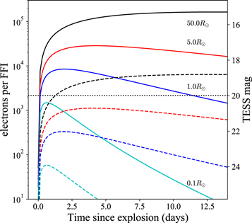
Figure 11. Light curves of Kasen (2010) models, converted to electrons per TESS FFI and TESS magnitudes. The models show the expected response of the SN ejecta shocked by colliding with a companion star—flux from the ejecta itself (powered by the decay of 56Ni) is not included. The light curves were calculated for a fiducial model with a viewing angle of 45°, an ejecta mass of 1.4 M⊙, a velocity of 104 km s−1, and an opacity of 0.2 cm2 g−1 (see Section 5). We show light curves for R = 0.1, 1.0, 5.0, and 50 R⊙ companions (from faintest to brightest) at either 50 Mpc (z ≈ 0.01, solid curves) or 200 Mpc (z ≈ 0.05, dashed curves). The horizontal line shows the typical 3σ detection limit for an 8 hr average of the FFIs. Within about ∼50 Mpc (z ≈ 0.01), we expect to be able to detect emission from a 0.1 to 1.0 R⊙ companion (see Section 6).
Download figure:
Standard image High-resolution imageIn summary, we have presented early-time light curves of SNe Ia from the first six sectors of the TESS primary mission, nine of which were amenable to analysis of the early rise. We fit rising power-law models and searched for signatures of any companion stars in these sources. Our main results are as follows:
- 1.We found a diversity of early-time light-curve shapes, although most of our SNe are consistent with fireball models with power-law indices β ≈ 2.0. Three out of nine SNe have a much lower rising power-law index with β ∼ 1.0.
- 2.We did not find obvious evidence for additional structures in the early-time light curves or companion signatures.
- 3.We placed upper limits on the radii of any companion stars of ≲20 R⊙ for five SNe and ≲4 R⊙ for two SNe. These constraints assumed a favorable viewing angle (<45°), as well as specific SN properties (ejecta mass, velocity, and opacity). The viewing angle assumptions imply that the odds of nondetection in this sample are 44% for companions with ≳20 R⊙ and 72% for companions with ≳4 R⊙, if such systems are actually commonplace. Thus, we cannot make inferences about the fraction of SNe Ia with non-degenerate companions. However, after its two-year mission, TESS has a 99% chance of observing enough SNe to either detect the signature of a companion star with R > 20 R⊙ in an SN Ia or set strong limits on the occurrence rate of such systems.
- 4.TESS is able to observe a companion signature for small companion stars (R < 4 R⊙) in an SN Ia within 50 Mpc and has a reasonable chance of doing so after about six years of operations.
We thank Saul Rappaport for discussions about binary systems and mass transfer and Marco Montalto for a discussion of TESS scattered-light signals at the TESS Science Conference I (2019 August).
This paper includes data collected by the TESS mission, which are publicly available from the Mikulski Archive for Space Telescopes and are described in Jenkins et al. (2016). Funding for the TESS mission is provided by NASA’s Science Mission directorate. This research has made use of NASA’s Astrophysics Data System, as well as the NASA/IPAC Extragalactic Database, which is operated by the Jet Propulsion Laboratory, California Institute of Technology, under contract with the National Aeronautics and Space Administration.
P.J.V. is supported by the National Science Foundation (NSF) Graduate Research Fellowship Program under grant No. DGE-1343012. K.Z.S. and C.S.K. are supported by NSF grants AST-1515876, AST-1515927, and AST-1814440. C.S.K. was also supported by a fellowship from the Radcliffe Institute for Advanced Studies at Harvard University. B.J.S., C.S.K., and K.Z.S. are supported by NSF grant AST-1907570. B.J.S. is also supported by NASA grant 80NSSC19K1717 and NSF grants AST-1920392 and AST-1911074. M.A.T. acknowledges support from the DOE CSGF through grant DE-SC0019323. The work of A.P. was supported in part by the GINOP-2.3.2-15-2016-00033 project, which is funded by the Hungarian National Research, Development, and Innovation Fund together with the European Union. T.D. acknowledges support from MIT’s Kavli Institute as a Kavli postdoctoral fellow.
Facility: TESS. -
Software: Matplotlib (Hunter 2007), NumPy (van der Walt et al. 2011), SciPy (Oliphant 2007), Astropy (Astropy Collaboration et al. 2018), limfit, 23 pysynphot (STScI Development Team 2013), SNooPy (Burns et al. 2011), ISIS (Alard & Lupton 1998).
Appendix A
In Appendix A, we show the original light curves of each SN and the auxiliary data used to identify and remove systematic errors. Figures 12–35 show the data for each SN—see Sections 3 and 3.1, and Figure 12 for more details.
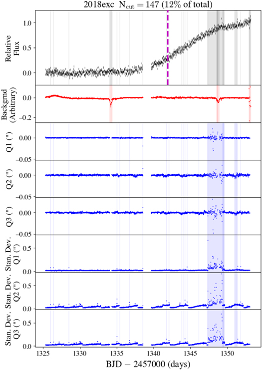
Figure 12. The light curve of SN 2018exc and the associated time series data used to identify unreliable photometry. The flux units are normalized relative to peak. The top panel shows the light curve (black lines) and 1σ uncertainties. The vertical purple line is the time of discovery. The shaded gray regions show the epochs that were removed based on the procedures defined in Section 3.1 (the same epochs are shown in the panels below). The next panel shows the time series of the local background estimated in a 4/8 pixel inner/outer annular region in the difference images. Three rounds of 5σ clipping were used to identify periods with rapidly changing or elevated backgrounds (see Section 3.1), which are highlighted by the shaded red regions. The panels labeled “Q1,” “Q2,” and “Q3” show the guiding offset quaternions in units of arcseconds; the Q1/Q2 components represent offsets along the TESS detectors’ rows/columns, while the Q3 direction represents spacecraft roll. The guiding offset data were rebinned from 0.5 s to the 30 minute time periods of each FFI and therefore show the average pointing of the spacecraft during that exposure. The last three panels show the standard deviation of the guiding offsets in each FFI bin. Three rounds of 5σ clipping were used to identify periods with increased jitter or large pointing offsets (see Section 3.1) and are highlighted by the shaded blue regions.
Download figure:
Standard image High-resolution image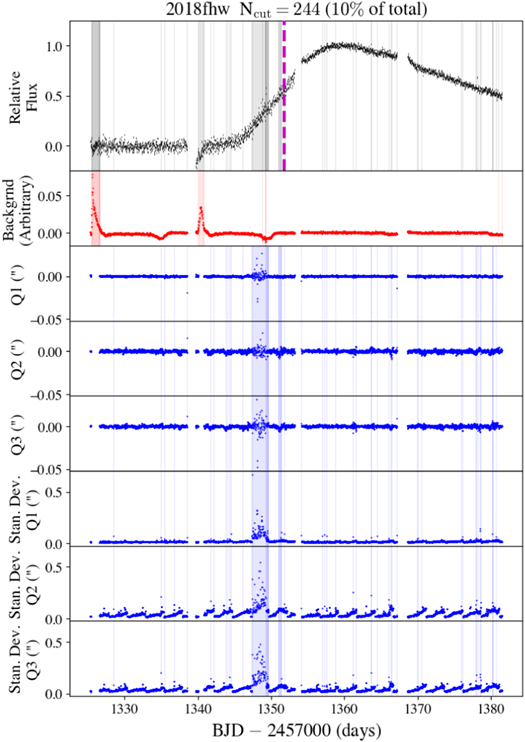
Figure 13. Same as Figure 12, but for SN 2018fhw.
Download figure:
Standard image High-resolution image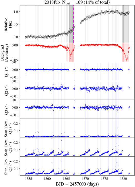
Figure 14. Same as Figure 12, but for SN 2018fub.
Download figure:
Standard image High-resolution image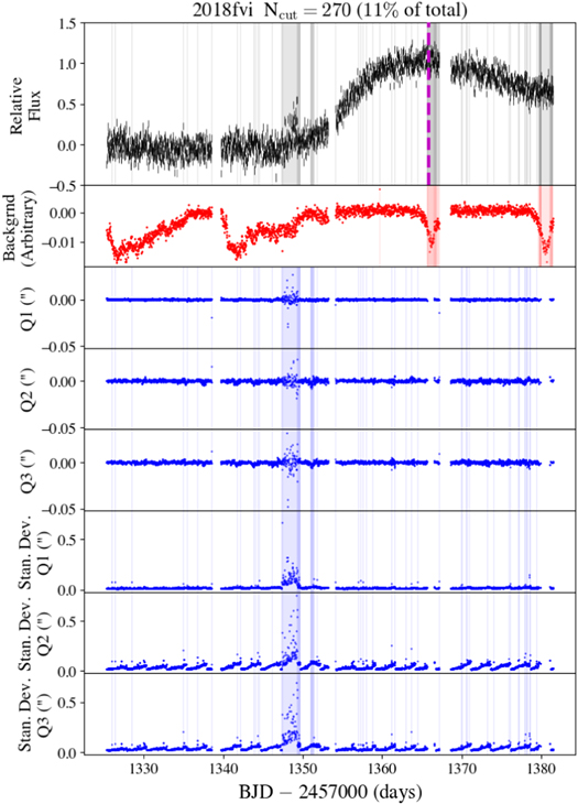
Figure 15. Same as Figure 12, but for SN 2018fvi.
Download figure:
Standard image High-resolution image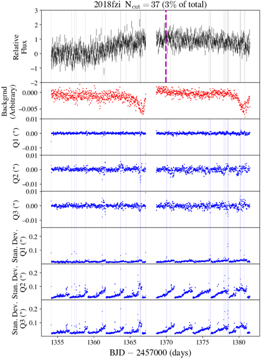
Figure 16. Same as Figure 12, but for SN 2018fzi.
Download figure:
Standard image High-resolution image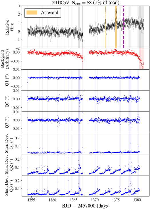
Figure 17. Same as Figure 12, but for SN 2018grv.
Download figure:
Standard image High-resolution image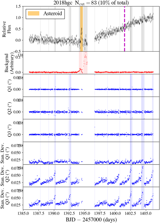
Figure 18. Same as Figure 12, but for SN 2018hgc.
Download figure:
Standard image High-resolution image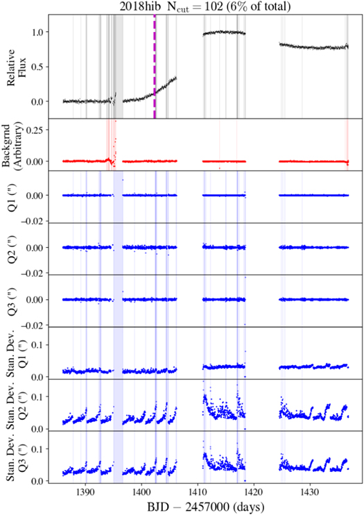
Figure 19. Same as Figure 12, but for SN 2018hib.
Download figure:
Standard image High-resolution image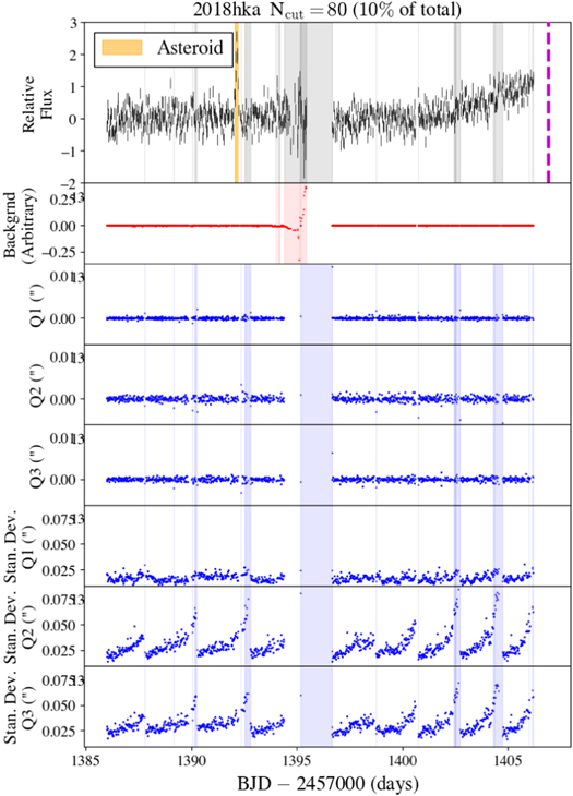
Figure 20. Same as Figure 12, but for SN 2018hkz.
Download figure:
Standard image High-resolution image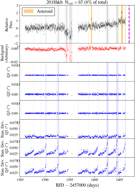
Figure 21. Same as Figure 12, but for SN 2018hkb.
Download figure:
Standard image High-resolution image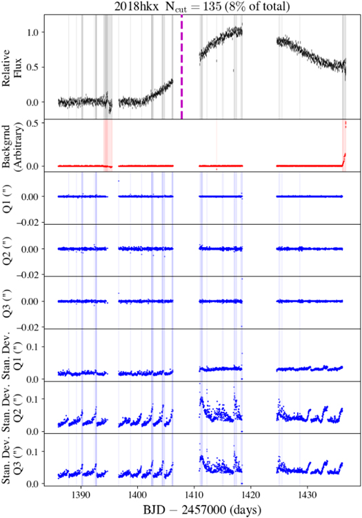
Figure 22. Same as Figure 12, but for SN 2018hkx.
Download figure:
Standard image High-resolution image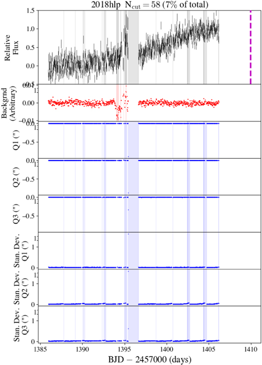
Figure 23. Same as Figure 12, but for SN 2018hlp.
Download figure:
Standard image High-resolution image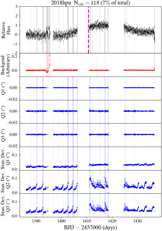
Figure 24. Same as Figure 12, but for SN 2018hpu.
Download figure:
Standard image High-resolution image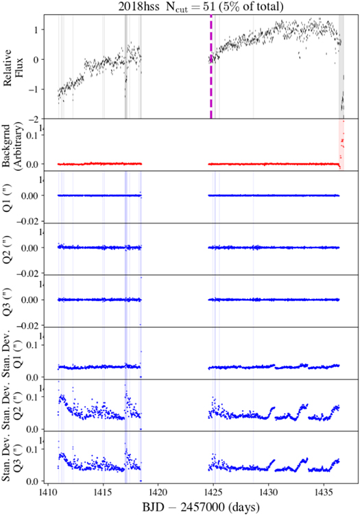
Figure 25. Same as Figure 12, but for SN 2018hss.
Download figure:
Standard image High-resolution image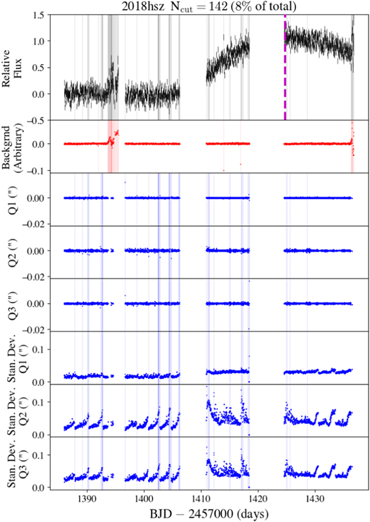
Figure 26. Same as Figure 12, but for SN 2018hsz.
Download figure:
Standard image High-resolution image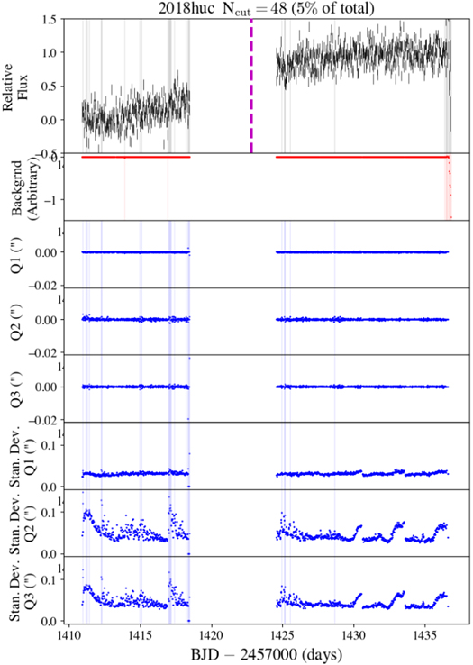
Figure 27. Same as Figure 12, but for SN 2018huc.
Download figure:
Standard image High-resolution image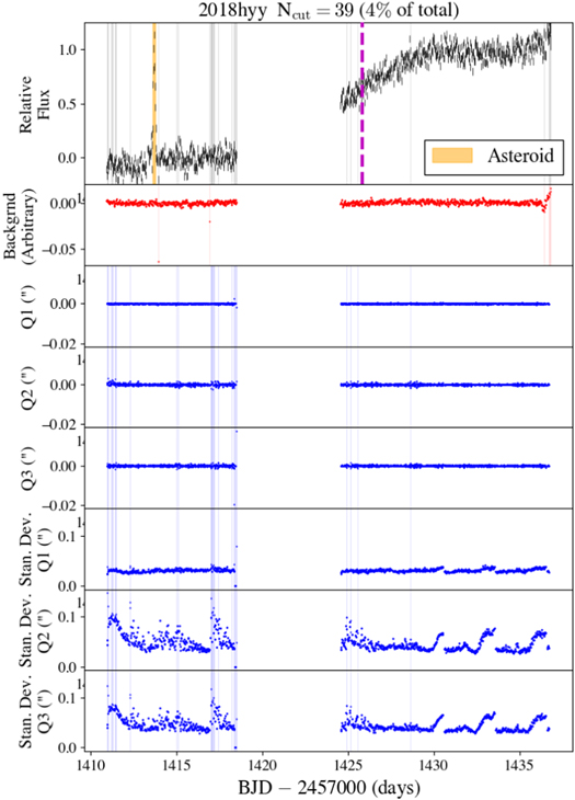
Figure 28. Same as Figure 12, but for SN 2018hyy.
Download figure:
Standard image High-resolution image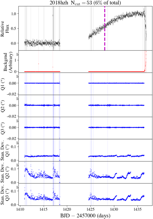
Figure 29. Same as Figure 12, but for SN 2018hzh.
Download figure:
Standard image High-resolution image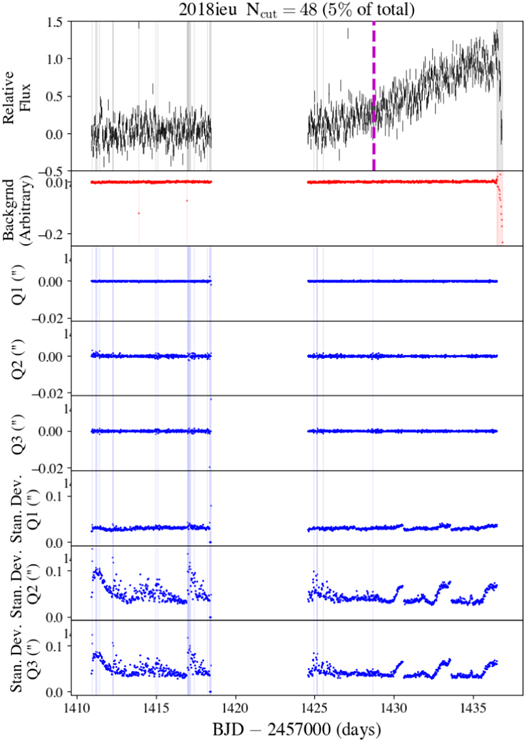
Figure 30. Same as Figure 12, but for SN 2018ieu.
Download figure:
Standard image High-resolution image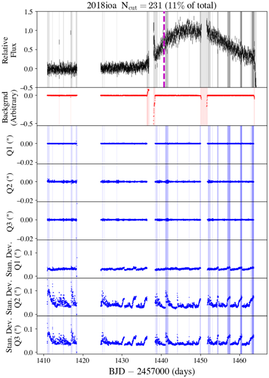
Figure 31. Same as Figure 12, but for SN 2018ioa.
Download figure:
Standard image High-resolution image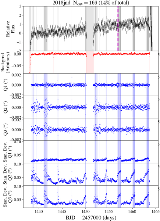
Figure 32. Same as Figure 12, but for SN 2018jnd.
Download figure:
Standard image High-resolution image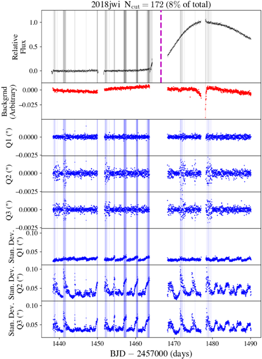
Figure 33. Same as Figure 12, but for SN 2018jwi.
Download figure:
Standard image High-resolution image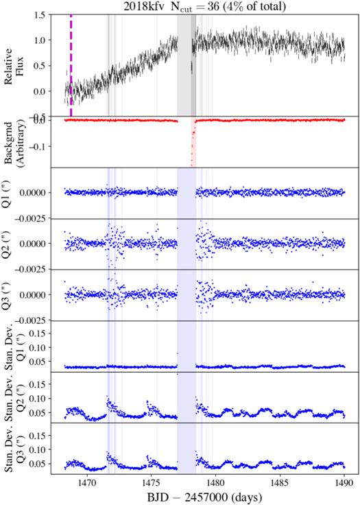
Figure 34. Same as Figure 12, but for SN 2018kfv.
Download figure:
Standard image High-resolution image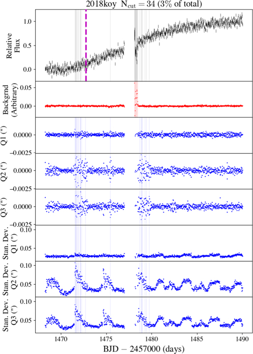
Figure 35. Same as Figure 12, but for SN 2018koy.
Download figure:
Standard image High-resolution imageAppendix B
In Appendix B, Figures 36–38 show SN light curves affected by nearby bright stars, as well as the light curves of the stars and fits used to correct the data.
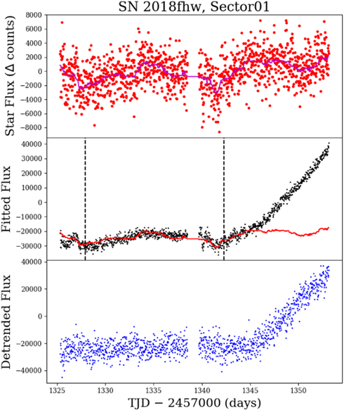
Figure 36. Detrending procedure for SN 2018fhw, Sector 1. This SN landed near a variable star that contaminated the photometric aperture. In the top panel, the red points show the star’s light curve, and the magenta line shows a smoothed model using a median filter. In the middle panel, the black points show the raw SN light curve, and the red line is the smoothed star model. The vertical dashed black lines show the period of time over which the star model was fit (with offset and scaling parameters). The blue points in the bottom panel show the corrected SN light curve. See Section 3.1 for more details.
Download figure:
Standard image High-resolution image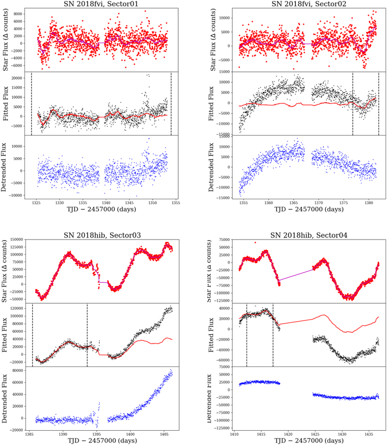
Figure 37. Same as Figure 36, but for 2018fvi and 2018hib.
Download figure:
Standard image High-resolution image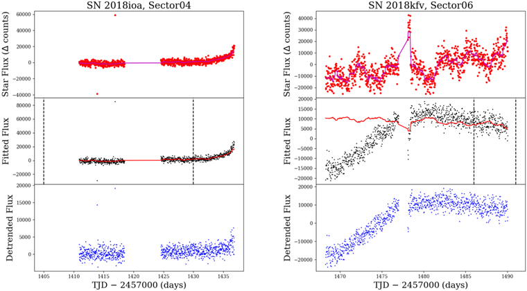
Figure 38. Same as Figure 36, but for SN 2018ioa and SN 2018kfv.
Download figure:
Standard image High-resolution imageAppendix C
In this section, we describe the Monte Carlo simulations used to test the grid search for companion signatures described in Section 5.2, and we define the 98% and 99.9% confidence intervals for χ2 used to place 2σ and 3σ limits on the separations/radii of companion stars in the TESS light curves.
We used the same fireball model for the SN explosion as in Section 5.1, which consisted of a sphere with a constant temperature of 104 K, an initial radius of 3 × 108 cm, and an expansion velocity of 109 cm s−1. The Kasen (2010) models have the same fiducial parameters used elsewhere in this work, with a viewing angle of 45°, an ejecta mass of 1.4 M⊙, a velocity of 104 km s−1, and an opacity of 0.2 cm2 g−1. We simulated each of the separations/radii of the companion models as in Section 5.1 (see Figure 4), with radii of 200 R⊙, 100 R⊙, 50 R⊙, 25 R⊙, 15 R⊙, 10 R⊙, 5 R⊙, and 1 R⊙ (or separations of 4.03, 2.02, 1.01, 0.50, 0.30, 0.20, 0.10, and 0.02 × 1013 cm, respectively). We also simulated the observed properties (such as the redshift and data gaps) of each SN presented in Section 5.2, namely, SN 2018exc, SN 2018fhw, SN 2018fub, SN 2018hib, SN 2018hkx, and SN 2018koy. In total, there were eight companion models for each of the six SNe, resulting in a total of 48 simulations.
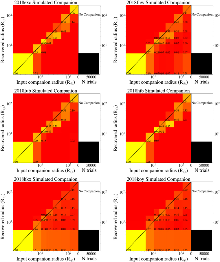
Figure 39. Left panels: 2D histograms showing the results of the Monte Carlo simulations that tested the fitting procedure detailed in Section 5.2. For each bin along the x-axis, 10,000 trials were run at that companion radius, while the bins along the y-axis show the distributions of the recovered companion radius. The fraction of trials in a given bin sum to unity along columns. Right panels: 1D histograms that show the recovered companion radius when no companion was actually present. In all cases, the minimum allowable companion radius was returned.
Download figure:
Standard image High-resolution image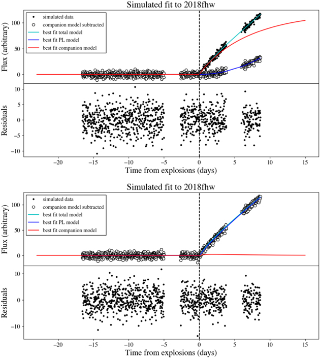
Figure 40. Examples of simulated data and fits for SN 2018fhw. The top panel shows a simulated companion model with an input radius of 223 R⊙. In this case, the grid search recovered the correct companion model. The bottom panel shows a different realization using the same input model, but here the fit recovered a small (1.1 R⊙) companion by compensating for the companion using a power-law index β = 0.86. This latter case accounts for the incorrectly recovered companion parameters in Figure 39. Such solutions were easy to identify and did not correspond to any of the results we found when fitting the TESS data in Section 5.2.
Download figure:
Standard image High-resolution image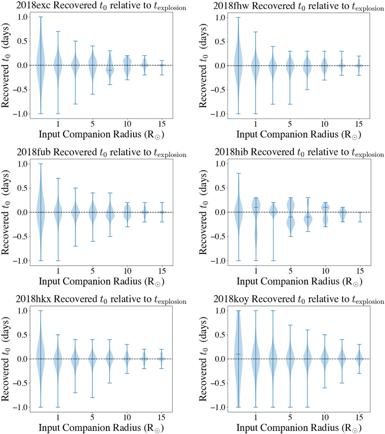
Figure 41. Distributions of recovered values of explosion times t0 for the Monte Carlo simulations described in Appendix C. The simulated light curves had t0 set to 0.0 days.
Download figure:
Standard image High-resolution image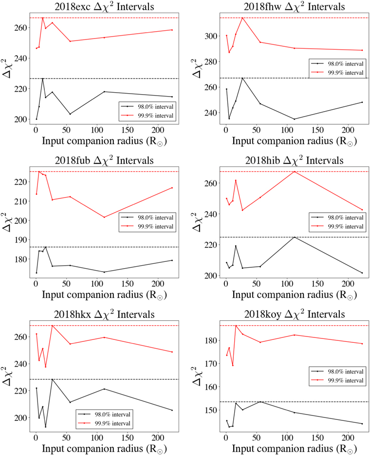
Figure 42. Ninety-eighth and 99.9th percentiles of the Δχ2 distributions for the Monte Carlo simulations described in Appendix C. The maximum value for each SN was adopted as the 2σ and 3σ statistical limits and was used to calculate the blue and red contours in Figure 7.
Download figure:
Standard image High-resolution imageFor each simulation, we converted the fireball and Kasen (2010) models to flux units by placing the object at the luminosity distance appropriate for each SN (see Table 1), calculating the TESS instrument response using synthetic photometry, and summing the two components to produce the simulated light curve. The light curves were then sampled at the TESS 30 minute FFI cadence, and sections of the light curve were removed to match the gaps in the observed light curves presented in Section 3. Finally, random Gaussian deviates were added to the synthetic light curves with amplitudes matching the observed pre-explosion light-curve dispersion. In units relative to peak, these scatter amplitudes were 0.04, 0.04, 0.03, 0.01, 0.03, and 0.05 for SN 2018exc, SN 2018fhw, SN 2018fub, SN 2018hib, SN 2018hkx, and SN 2018koy, respectively. In this way, the synthetic data closely matched the observed properties of the light curves, including their noise properties and sampling pattern.
After constructing the synthetic light curves, we performed three fits. First, we fit a power-law model of the form given in Equation (1). Second, we added a Kasen (2010) companion component to the power-law model and performed a grid search over the companion separation/radius and t0 to find the best-fit χ2. For each combination of companion separation/radius and t0, we first subtracted the Kasen (2010) model from the observed light curve and then fit a power-law model optimizing A, β, and B in Equation (1) (with t0 held fixed) so as to minimize χ2. We experimented with the spacing of the grid in companion separations/radii and t0, and found that the following parameters worked for our fits:
- 1.ten logarithmically spaced companion models between 1.1 R⊙ and 223 R⊙ (separations between 0.02 and 4.00 × 1013 cm, respectively), which translates into a grid of 1.1, 2.0, 3.6, 6.4, 11.7, 21.0, 38.0, 68.3, 123.2, and 223 R⊙;
- 2.t0 spaced every 0.1 days (2.4 hr) from −1 to +1 day relative to the value of t0 determined in the initial power-law fit.
As mentioned in Section 5.2, we used a finer grid of 20 logarithmically spaced companion separations and expanded the range of t0 from −2 to +5 days around the initial estimate of t0. In the third and final fit, we performed the same grid search but on a synthetic light curve with no companion model. We performed 10,000 iterations for each of the 48 simulations with different realizations of the measurement noise and recorded the best-fit χ2 from our grid search and the corresponding model parameters.
In Figure 39, we show 2D histograms of the recovered companion radius as a function of input companion radius for each SN. There was good correspondence between the input and recovered radii. For SN 2018exc, SN 2018hib, and SN 2018fub, the highest-probability recovered radius matched the input radius, at least to the closest bin of the grid search. For SN 2018exc, SN 2018hib, and SN 2018fub there was also a smaller but non-negligible probability that the recovered radius was off by one grid step toward a smaller companion radius than the true value. For SN 2018fhw, SN 2018hkx, and SN 2018koy (and in some rare cases, SN 2018fub), a range of possible companion radii were recovered for the largest simulated companions; in fact, for SN 2018hkx and SN 2018koy recovering a small companion with a radius of <1.1 R⊙ was more likely than recovering the true companion radius (>50 R⊙). Inspection of these solutions showed that the fits were driven by a low power-law index, with β < 1.0, which mimics the dominant companion light curve at early times. Thus, there is a degeneracy in early-time SN Ia light curves between intrinsically low values of β and large companions. An example of this degeneracy is shown in Figure 40. No such fits were found for the real TESS data in Section 5.2. It is somewhat unclear why this effect was not seen in SN 2018exc, SN 2018hib, or (to some extent) SN 2018fub, although it is probably related to individual noise properties, sampling patterns, and time ranges over which to fit a particular light curve. An interesting corollary of this result is that there may be an optimum time range over which to fit early-time Type Ia light curves (i.e., up to a larger or smaller fraction of the peak flux than the 40% adopted here) in order to find signatures of companion stars, but determining if this is the case is beyond the scope of this work.
The companion radius recovered in our third set of fits, when no companion model was present in the simulated light curves, is shown by the 1D histograms in the right panels of Figure 39. In all cases, our procedure returned the minimum allowable companion radius of the grid search.
Figure 41 shows the distributions of the recovered values of t0 for each input companion radius and each SN. For small values of the input companion radius, t0 was poorly constrained. This result is expected, because a very small companion signature will be comparable to the measurement noise and have a small effect on the final fit, while the parameters A and β can compensate for changes in t0. However, as the input companion radius increased, the distributions of t0 became narrower and more accurate, showing how the effects of large companions on the light curve are difficult to hide at early times. For the simulations with no companion signature model, the distributions of t0 were well constrained but biased to >0.5 days.
Finally, we used the distributions of χ2 to identify the 2σ and 3σ statistical limits that could be placed on the model parameters in the grid search. First, we calculated  for all 1000 trials of each simulation. We then used the 98th and 99.9th percentiles of the distributions of Δχ2 for each simulation to define the statistical 2σ and 3σ limits. Figure 42 shows these limits for all SNe as a function of input model companion separation. We adopted the largest Δχ2 intervals across the input companion separation/radius for the final 2σ and 3σ statistical limits. Table 8 gives the values of Δχ2 used for each SN. These intervals were transferred to the TESS data by finding the model with the minimum χ2 value in the grid search and adding the 2σ and 3σ Δχ2 values. The contours of these values of χ2 are shown in Figure 7. Any models with χ2 values outside of these χ2 contours arise by chance 2% or 0.1% of the time.
Table 8. Δχ2 Confidence Intervals
| Name | 98% Δχ2 | 99.9% Δχ2 |
|---|---|---|
| SN 2018exc | 230 | 277 |
| SN 2018fhw | 285 | 325 |
| SN 2018fub | 200 | 236 |
| SN 2018hib | 239 | 285 |
| SN 2018hkx | 232 | 274 |
| SN 2018koy | 157 | 190 |
Download table as: ASCIITypeset image
Footnotes
- 17
Sectors 14–16 and 24–26 are exceptions; see https://tess.mit.edu/observations.
- 18
- 19
- 20
The PRF models are available at https://archive.stsci.edu/missions/tess/models/prf_fitsfiles/.
- 21
The guiding quaternions are available at https://archive.stsci.edu/missions/tess/engineering/.
- 22
If we had instead fit this object up to 40% of the peak flux, we would have found t0 = 1339 ± 1.68 and β = 3.17 ± 0.66. This fit has larger uncertainties than fitting up to 60% of the flux but is consistent with the values in Table 4. However, a fit up to 40% of the flux would put t0 just at the end of a large data gap, which is unlikely to be an accurate estimate of the time of explosion.
- 23