Abstract
Filaments are ubiquitous structures in molecular clouds and play an important role in the mass assembly of stars. We present results of dynamical stability analyses for filaments in the infrared dark cloud G14.225−0.506, where a delayed onset of massive star formation was reported in the two hubs at the convergence of multiple filaments of parsec length. Full-synthesis imaging is performed with the Atacama Large Millimeter/submillimeter Array to map the  emission in two hub-filament systems with a spatial resolution of ∼0.034 pc. Kinematics are derived from a sophisticated spectral fitting algorithm that accounts for line blending, large optical depth, and multiple velocity components. We identify five velocity coherent filaments and derive their velocity gradients with principal component analysis. The mass accretion rates along the filaments are up to
  and are significant enough to affect the hub dynamics within one freefall time (∼105 yr). The
  filaments are in equilibrium with virial parameter αvir ∼ 1.2. We compare αvir measured in the
  filaments,
  filaments, 870 μm dense clumps, and 3 mm dense cores. The decreasing trend in αvir with decreasing spatial scales persists, suggesting an increasingly important role of gravity at small scales. Meanwhile, αvir also decreases with decreasing nonthermal motions. In combination with the absence of high-mass protostars and massive cores, our results are consistent with the global hierarchical collapse scenario.
Original content from this work may be used under the terms of the Creative Commons Attribution 3.0 licence. Any further distribution of this work must maintain attribution to the author(s) and the title of the work, journal citation and DOI.
1. Introduction
How accretion proceeds around young star clusters affects the mass growth of protostars and is critical to the understanding of the origin of the initial mass function (IMF). The lack of observational characterization of young cluster-forming regions precludes a unified theoretical scenario to explain star formation across several orders of magnitude in mass and scales. Recent Herschel observations reveal that parsec-scale filaments are prevalent in molecular clouds (e.g., Andre et al. 2010; Molinari et al. 2010; Arzoumanian et al. 2011, 2013; Palmeirim et al. 2013). Young stellar groups are often found in dense clumps of column density exceeding  at the convergence of multiple filaments of parsec length, namely “hub-filament systems” (Myers 2009a; Liu et al. 2012, 2015; Peretto et al. 2013, 2014; Lu et al. 2018; Williams et al. 2018). On the basis of core accretion scenarios (e.g., Shu 1977; McKee & Tan 2003), theoretical models have gradually incorporated accretion from the surrounding clumps (e.g., Bate & Bonnell 2005; Wang et al. 2010; Myers 2011, 2013). Cores embedded in denser clumps benefit by accretion from the filamentary environment so as to prolong the accretion time for growing massive stars (Myers 2009b). Meanwhile, numerical simulations of colliding flows and collapsing turbulent clumps grow massive protostars from low-mass stellar seeds by feeding gas along the dense filamentary streams converging toward the 0.1 pc size hubs with detectable velocity gradients along the filaments (e.g., Wang et al. 2010; Gómez & Vázquez-Semadeni 2014; Smith et al. 2016). Although filaments are expected in colliding flows, their origin and internal structures remain debatable (Moeckel & Burkert 2015; Smith et al. 2016; Clarke et al. 2017). To date, only a few spectral line observations have been conducted to trace the hypothesized accretion flows along filaments, presumably toward the center of gravity, where protoclusters are located (e.g., Liu et al. 2012; Kirk et al. 2013; Peretto et al. 2013; Lu et al. 2018).
At a distance of  (Xu et al. 2011), the infrared dark cloud (IRDC) G14.225−0.506 (hereafter G14.2) is part of the remarkable IRDC complex, M17 SWex (Figure 1(a); Povich & Whitney 2010), which was first discovered by Elmegreen & Lada (1976) in the CO map as a large (67 pc ×17 pc) and massive (∼3 × 10⁵ M☉) molecular cloud complex extended parallel to the Galactic plane southwest of the well-known giant H ii region M17. In the most extincted part of M17 SWex, the
  emission reveals a network of filaments associated with two warmer (Trot ∼ 15 K) hubs, hub-N and hub-S, at the convergence of multiple cold, velocity coherent filaments (∼10 K) of parsec lengths at distinct velocities (Busquet et al. 2013). The velocity dispersion in hubs is a factor of ∼2 broader than that in filaments. The larger velocity dispersion in the hubs may be due to higher temperature, star formation activities, colliding filaments (Wang et al. 2010), or longitudinally collapsing filaments (Peretto et al. 2014). Analyses of young stellar objects (YSOs) based on near- and mid-infrared Spitzer photometry data together with the Chandra X-ray census (for diskless YSOs) reveal a rich population of intermediate-mass YSOs without commensurate, simultaneous massive star formation (Povich & Whitney 2010; Povich et al. 2016). Such a conspicuous deficit of O-type massive protostars implies that either the IRDC G14.2 may be an example of a distributed star formation mode with OB clusters dominated by intermediate-mass stars, or its massive hubs/cores are still in the process of accreting ambient material to nurture massive protostars. In the latter case, the high-mass tail in the protostar mass function will arise later in time (Bonnell & Bate 2006; Myers 2009b; Vázquez-Semadeni et al. 2017). Ohashi et al. (2016) have performed a dense core survey in IRDC G14.2 using the 3 mm continuum emission (angular resolutions of ∼3″ × 2″ and a sensitivity of 0.28 M☉) in two mosaic fields covering the two hubs and their associated networks of filaments (see Figure 1(b)). The maximum mass of the prestellar or protostellar cores (≲22 M☉) suggests a scenario of forming high-mass stars in prestellar cores by accreting a significant amount of gas from the surroundings or prolonging the accretion from protostellar cores to intermediate-mass YSOs. The hubs contain more mass and have the potential to nurture massive stars. The total gas mass estimated by Ohashi et al. (2016) is 1400 M⊙ in the hub-N and 960 M⊙ in the hub-S. Assuming a star formation efficiency of 30% and the IMF from Kroupa (2001), we estimate the expected maximum stellar mass to be 27 M⊙ in the hub-N and 21 M⊙ in the hub-S (apply Equation (2) in Sanhueza et al. 2017). If so, IRDC G14.2 is one of the most ideal systems to characterize the initial conditions of massive star formation.
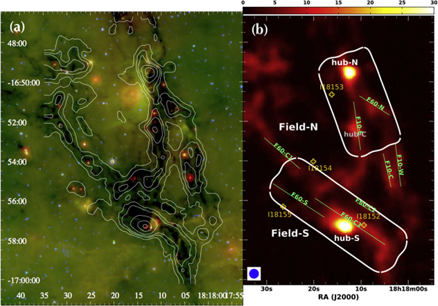
Figure 1. (a) Archival Spitzer  (blue/green/red) three-color composite image of G14.225−0.506 overlaid with the
  integrated intensity map (contours) observed with the IRAM 30 m Telescope (G. Busquet et al. 2019, in preparation). Contour levels are (4, 8, 12, 24, 48, and 72) × σ, where the rms noise level is
  . (b) ALMA mosaic fields, Field-N and Field-S (white boxes), overlaid on the same
  integrated intensity map (color scale) as in (a). The two massive star-forming hubs, hub-N and hub-S, are labeled. Yellow open crosses indicate the IRAS sources in the field of view. Green lines with labels indicate the positions of the previously identified
  filaments (Busquet et al. 2013).
Download figure:
Standard image High-resolution imageTo trace quiescent gas kinematics in G14.2, we choose to map emission of the molecular ion,  , which has a much higher critical density,
  , and a lower upper-level energy,
  , than the
  line with
  and Eup = 23.4 K (Shirley 2015). The multiple-spin coupling induced by the two nitrogen nuclei in the molecular ion,
  , gives rise to splitting of the J = 1−0 line into seven closely spaced hyperfine components (Green et al. 1974), which are often observed in high-mass star-forming regions and IRDCs as a triplet of lines (Caselli et al. 1995; Shirley et al. 2005; Sanhueza et al. 2012). Only one isolated component,
  , is well separated from the other six hyperfine components and can be used to directly trace gas kinematics without the need to fit all the components. This isolated component, however, is fairly weak and has a relative intensity of merely 1/9 ≃ 0.11 of the total intensity (Mangum & Shirley 2015).
In this paper, we present full-synthesis images of the  line obtained with the Atacama Large Millimeter/submillimeter Array (ALMA) in the two mosaic fields. The continuum counterpart of the data were previously reported by Ohashi et al. (2016). Details of
  line observations are described in Section 2. The morphology of dense molecular gas and its relation with the embedded YSOs are discussed in Section 3. Identification and kinematics analyses of filaments are described in Section 4. We then discuss the main results in Section 5, and conclude in Section 6.
2. Observations
The IRDC G14.2 was observed with the ALMA 12 m Array on 2015 April 25 in the C34-2/1 configuration with a total of 37 antennas and with the Atacama Compact Array (ACA; 7 m Array antennas) on 2015 April 30 and May 4, and on 2016 May 15 and June 4 with a total of 10 antennas (Cycle 2 and 3 programs, Project ID: 2013.1.00312.S and 2015.1.00418.S; PI: Vivien Chen). Observations with the total power (TP) array were conducted from 2016 May 14 to May 20 in multiple sessions. The total number of the 12 m array pointings is 57 in Field-N and 67 in Field-S (Figure 1(b)). The duration of all the 12 m array observation, including time for calibration, is roughly 1.7 hr. All observations employed the Band 3 receivers with an instrumental spectral resolution of 31 kHz centered at the rest frequency of 93.1738 GHz for the  transition. The system temperatures ranged from 60 to 90 K. The projected baselines, including both 7 and 12 m arrays, ranged from 2.6 to
  , equivalent to 0
85 to 35″. The quasars J1733−1304 and J1924−2914 were observed for bandpass, phase, and amplitude calibration. Flux calibration was performed using Neptune and Ceres. The uncertainty of absolute flux calibration is 5% in Band 3 according to ALMA Cycle 2 Technical Handbook. The reduction and calibration of the data were done with CASA version 4.3.1, 4.5.3, and 4.7.0 (McMullin et al. 2007) using the standard procedures, and the data were delivered from the East Asian ALMA Regional Center. The visibility data were then exported in FITS format to the MIRIAD package for imaging reconstruction with the robust parameter equal to zero. For a better sensitivity, visibility data were smoothed from an instrumental spectral resolution of 0.1 to
 before making images. The TP image cubes were used as default images when performing the maximum entropy deconvolution. To avoid undesired distortion in the following statistical analyses, the spectral line image in each mosaic field was restored with a circular beam size equal to the solid angle of the Gaussian synthesized beam. The beam size of the final image is 3
48 for Field-N and 3
15 for Field-S, and the pixel size is 0
3. The rms noise level per channel is
 (0.32 K) in Field-N and
  (0.32 K) in Field-S. Integrated intensity maps are also generated with visibilities averaged within a velocity range of
  and
and  for Field-N and Field-S, respectively. The respective rms noise level is 1.30 and
  in Field-N and Field-S.
3. Results
Figures 2 and 3 show the integrated intensity maps of the  emission in the two mosaic fields along with their intensity-weighted velocity (moment 1) maps generated solely with the isolated hyperfine component (
 ). The intensity-weighted velocity maps are computed with a clip value of 2.5σ over a velocity range of
  for Field-N and
  for Field-S. Similar to the ammonia emission reported by Busquet et al. (2013), the
  emission also shows a network of filaments, where hubs are located at the intersection of multiple filaments. With much improved angular resolution of ∼3
5 (equivalent to 0.034 pc), we are able to resolve structures down to their thermal Jeans length of 0.06 pc (assuming a density of
 at 10 K). Both hubs show extended, elongated structures connecting to their surrounding filaments. The velocity distributions in both fields show a general flow pattern (Figures 2(b) and 3(b)). An overall velocity gradient is clearly revealed in each mosaic field, suggesting inflow motions along filaments, most likely toward the center of gravity, where the hubs are located. Because our spectra show multiple velocity components in many positions, one should regard the intensity-weighted velocity maps as weighted mean velocity distribution of the actual complicated kinematics in the regions. In Field-N, gas velocity decreases from
  in the south to
  in the north. Two fairly distinct velocity distribution are found in Field-S, where velocity increases from
  in the northeast to
  in the southwest.
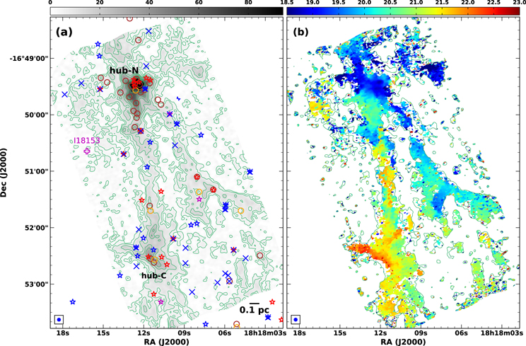
Figure 2. (a) ALMA  integrated intensity map of Field-N showing a remarkable filamentary morphology in dense gas. The dominant star-forming core, hub-N, is associated with dense cores, embedded YSOs, and several prominent filaments in this region. One more hub candidate, hub-C, shows stronger
  emission and is also associated with a group of YSOs and two dense cores. Contour levels are (3, 5, 10, 15, 20, 30, 40, 50, 60, 80, 100) × σ, where the rms noise level is
  . Dense cores identified in the 3 mm continuum emission and dense clumps identified in the 870 μm continuum emission (Ohashi et al. 2016) are shown as brown and orange open circles, respectively. The magenta cross marks the position of IRAS 18153−1651. YSOs with AV > 20 mag are also shown (Povich et al. 2016): spectral energy distribution (SED) classification in stage 0/I sources (red stars), stage II/III (blue stars), and ambiguous (magenta stars). Blue crosses mark the positions of X-ray sources associated with the cluster (Povich et al. 2016). (b) Intensity-weighted velocity (moment 1) map of the isolated hyperfine component (
 ) of
) of  emission. One can see a generally increasing trend in velocity from north to south. Each filament appears in a slightly different velocity range.
Download figure:
Standard image High-resolution image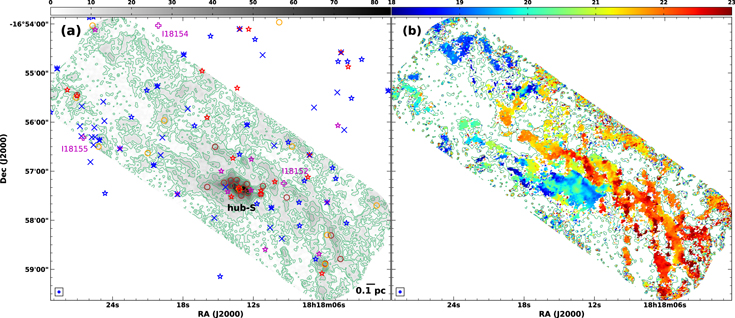
Figure 3. (a) ALMA  integrated intensity map of Field-S. The dominant star-forming core, hub-S, is associated with dense cores, embedded YSOs, and several prominent filaments in this region. Contour levels are (3, 5, 10, 15, 20, 30, 40, 50, 60, 80) × σ, where the rms noise level is
  . The magenta crosses mark the positions of IRAS 18155−1657, IRAS 18152−1658, and IRAS 18154−1655. All other symbols are the same as in Figure 2. (b) Intensity-weighted velocity (moment 1) map of the isolated hyperfine component (
 ) of
) of  emission. One can see two fairly distinct velocities between the northeast part and southwest part of the cloud.
Download figure:
Standard image High-resolution imageIn general, deeply embedded YSOs (red stars as stage 0/I sources; Povich et al. 2016) are found to be associated with hubs and filaments, while evolved YSOs (blue stars as stage II/III and blue crosses as X-ray sources; Povich et al. 2016) appear more distributed in the regions. Dense cores identified in the continuum studies (brown open circles; Ohashi et al. 2016) are preferentially located in hubs, and just a few are in filaments. This perceptible association of dense cores and deeply embedded YSOs with filaments, particular in the vicinity of the hubs, assures that filaments are part of star formation processes instead of occasional overdense features in clouds. Filaments may participate in star formation in two ways: fragmentation into cores with nearly equal spacings (e.g., Zhang et al. 2009, 2015; Wang et al. 2011; Naranjo-Romero et al. 2012) or longitudinal accretion flow along the axis (e.g., Kirk et al. 2013; Peretto et al. 2013; Contreras et al. 2016; Lu et al. 2018). On the basis of the  gas flow motion toward the hubs and positions of the continuum dense cores not being regularly spaced (Figures 2 and 3), the filaments in IRDC G14.2 are more inclined to mass accretion into the hubs rather than fragmentation into cores. Yet the two aspects are not mutually exclusive and may occur simultaneously.
In addition, a small group of YSOs and two dense cores appear to be associated with a hub candidate, hub-C, at convergence of two elongated structures with different orientations (Figure 2). Similar to hub-N and hub-S, this candidate hub also shows warm and compact  emission (Busquet et al. 2013), whose upper-level energy is 65 K. The rotational temperature in hub-C ranges from 15 to 25 K (G. Busquet 2019, private communication).
The general gas kinematics are shown in velocity channel maps with step of  (Figures 4 and 5). In addition, velocity channel maps of the isolated component with a spectral resolution of
  (Figures 18 and 19) and the corresponding animations (Figures 4 and 5) are available. A few filaments are easily identified as persistent structures across consecutive velocity channels with clear velocity gradients. The two prominent hubs, hub-N and hub-S, both exhibit large velocity spreads of more than
  . Hence, we specify the spatial extent of the hubs to be regions with emission in more than 10 consecutive channels, equivalent to
  , and with intensities greater than 3σ in the isolated hyperfine component.
Figure 4. Velocity channel maps of the isolated hyperfine component ( ) of
) of  emission in Field-N with step of
  . To show filamentary structures, the grayscale is saturated in hub-N. The two dominant filaments are well separated in space and velocity. The velocity channel maps used for our spectral analysis with step of
  are available as a figure set (Figure 18). An animated version of the velocity channel maps in step of
  is available. The video duration is 8 s.
(An animation of this figure is available.)
Download figure:
Video Standard image High-resolution imageFigure 5. Velocity channel maps of the isolated hyperfine component ( ) of
) of  emission in Field-S with step of
  . To show filamentary structures, the grayscale is saturated in hub-S. Multiple filaments are likely present in this field. The velocity channel maps used for our spectral analysis with step of
  are available as a figure set (Figure 19). An animated version of the velocity channel maps in step of
  is available. The video duration is 8 s.
(An animation of this figure is available.)
Download figure:
Video Standard image High-resolution image4. Analyses
4.1. Filament Identification
We use the publicly available filament finding package FilFinder (Koch & Rosolowsky 2015)14 skeletons. FilFinder isolates filamentary structures by creating a mask with adaptive threshold, where a valid pixel must have intensity greater than the median of the neighborhood around it. An object also needs to have an aspect ratio larger than 5 to be considered as a branch or filament. Each filament mask is then reduced to a skeleton using medial axis transform. The algorithm then drives the shortest path between each pair of end points and finds the longest path in a connected path network to be the final filament spine. The remaining branches are pruned, leaving the dominant spine for further analyses. The sum of branch lengths for this dominant spine is defined to be the length of the filament, ℓ.
To extract skeletons in our mosaic fields, we first select persistent structures in consecutive velocity channels (at least three channels for local structures and eight channels for the entire filament) and generate integrated intensity maps that are most optimal to individual structures. However, this approach restricts us to use solely the isolated hyperfine component, which does not suffer from line blending but is merely ∼1/9 in the total intensity. Although the signal-to-noise ratio is lower, we are able to extract skeletons, which are relatively brighter features in filaments. The mask is prepared with a flattened percentage of 90% and a minimum intensity to be included (glob_thresh) at 60% for field-N and 40% for field-S. We prune branches shorter than 1 pc to avoid confusion in the margins of the mosaic fields. The performance of FilFinder is fairly robust. The spine identification does not vary drastically unless the parameters are deviated far from the default values. In addition, we terminate a spine when it enters one of the two prominent hubs, whose spatial extent is defined as a region with emission higher than 3σ in more than 10 channels (see Section 3). This is to avoid a hub connecting all its associated filaments as one whole kinetic ensemble structure. In total, FilFinder identifies five  filaments (Figure 6): two in Field-N and three in Field-S. Because these filaments spatially overlap with the ammonia filaments (Busquet et al. 2013), we simply follow the nomenclature to label the
  filaments and list their basic properties in Table 1. The length of the
  filaments, ℓ, is in the range of 1.02–3.22 pc with a mean value of 2.0 pc. We consider these projected filament lengths to be the lower limits of the actual filament lengths in 3D space. Note that some previously identified
  filaments are not labeled in Figure 6 if they are just partially present in the periphery of our mosaic fields. The emission contrast of a filament to its surroundings varies among filaments. Filament F10-E shows the largest contrast, while F60-S and F60-C2 are clumpy and diffuse.
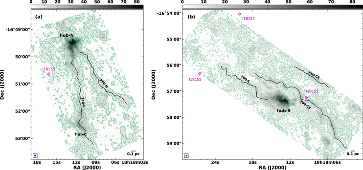
Figure 6. (a) Filaments identified with the FilFinder package in Field-N overlaid on the integrated intensity map. The magenta cross marks the positions of IRAS 18153−1651. Contour levels follow those in Figure 2. (b) Identified  filaments in Field-S overlaid on the integrated intensity map. The magenta crosses mark the positions of IRAS 18155−1657, IRAS 18152−1658, and IRAS 18154−1655. Contour levels follow those in Figure 3.
Download figure:
Standard image High-resolution imageTable 1. Filament Length and Width
| Filament | ℓ(pc)a | w (pc) | p | υ ( )b )b
|
|---|---|---|---|---|
| Field-N | ||||
| F10-E | 2.26 | 0.07 ± 0.05 | 2.2 ± 0.6 | 19.7–22.9 |
| F60-N | 1.81 | 0.09 ± 0.07 | 3.6 ± 2.5 | 18.9–21.2 |
| Field-S | ||||
| F60-C3 | 3.22 | 0.05 ± 0.03 | 2.5 ± 0.6 | 20.9–23.3 |
| F60-S | 1.67 | 0.05 ± 0.06 | 2.5 ± 1.5 | 18.1–21.1 |
| F60-C2 | 1.02 | 0.07 ± 0.08 | 2.5 ± 1.7 | 20.9–22.5 |
Notes.
aFilament projected length on the sky regarded as the minimum length. bVelocity range used to identify the filament.Download table as: ASCIITypeset image
4.2. Filament Width
Following the analyses of previous studies of filaments (e.g., Arzoumanian et al. 2011; Palmeirim et al. 2013), we analyze the integrated intensity profile of the  emission with an idealized cylindrical model described by a Plummer-like function:

where ρc is the central density of the filament, p is the power-law exponent at large radii, Ap is a finite constant factor, and Rflat is the inner flat portion of the density profile. The filament width is given by  . In the special case of an isothermal filament in hydrostatic equilibrium, Ostriker (1964) found p = 4,
  , and Rflat equal to the thermal Jeans length at the center of the filament. Early studies with Herschel continuum data found p = 2 and w = 0.1 pc (Arzoumanian et al. 2013; Palmeirim et al. 2013). This r−2 density profile has also been reproduced in numerical models of filamentary clouds with helical magnetic fields and turbulent pressure of the surrounding interstellar medium (Fiege & Pudritz 2000). Yet steeper density profiles with p = 2.7–5.1 have also been reported in a number of filaments (Nutter et al. 2008; Hacar & Tafalla 2011; Pineda et al. 2011; Monsch et al. 2018).
To find the filament width, w, we apply the publicly available filament profile builder package RadFil (Zucker et al. 2018a, 2018b)15
to the integrated intensity maps of the  emission. Given a filament spine together with a filament mask, RadFil first smooths the input spine pixels to a continuous version of the spine, i.e., a basis spline, and then creates cuts according to the positions and the first derivative of the basis spine to build intensity profile across the filament. The algorithm allows shifting the profile by searching for the pixel with the peak intensity along each cut but inside the filament mask. Once the radial profiles along all the cuts are computed, RadFil fits a given profile function, such as the Plummer function, on the average profile of the entire ensemble of cuts. We produce a mask of 0.1 pc width following each individual filament spine to confine the search for the peak intensity pixels so the algorithm will not be confused by nearby branches or filaments. Cuts are taken every 12 pixels (samp_int=12), which are roughly equal to the beam size. RadFil also allows a background emission subtraction before performing the profile fit. A first-order polynomial fit is applied to the background emission model for proper subtraction. The background model is obtained with data in regions between 0.2 and 0.8 pc from the spine. The range is selected to obtain most of the available data on the two sides of individual filaments. We also mask out hubs to reduce the bias in the background subtraction when computing the profiles along cuts.
The widths from the optimized fits are given in Table 1. As an example, the profile fit along the spine of filament F10-E is shown in Figure 7. The filament widths are in the range of 0.05 to 0.09 pc, with a mean value of 0.07 pc, which is smaller than but comparable to the characteristic width of 0.1 pc reported in the previous Herschel studies with dust emission (e.g., Arzoumanian et al. 2011, 2019; Palmeirim et al. 2013). Narrow widths down to ∼0.02 pc have also been reported in a number of filaments observed with molecular gas (e.g., Pineda et al. 2011; Hacar et al. 2018; Monsch et al. 2018). Meanwhile, theoretical studies have pointed out possible bias introduced by the method for interpreting the data. Filaments are made up of preexisting short subfilaments, and the widths may have a broader distribution instead of being a constant (Smith et al. 2014). The measured width is also likely to be affected by the choice of parameters (Panopoulou et al. 2017).
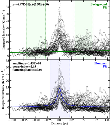
Figure 7. Plummer function fit with the integrated intensity cuts across filament F10-E using the Python package RadFil. (Top) Background model with a first-order polynomial using data between 0.3 and 0.7 pc from the spine (green shaded regions bounded by vertical green dash line). Thick green line shows the best-fit background. Thin black lines show the profiles of the entire ensemble of cuts. (Bottom) The best-fit Plummer profile (thick blue line) to the background-subtracted profiles (thin black lines) within 0.2 pc from the spin.
Download figure:
Standard image High-resolution image4.3. Spectral Fits for Hyperfine Structures
We derive the kinematics pixel by pixel with a sophisticated spectral model that accounts for multiple velocity components, as well as optical depth and line blending. Along each line of sight (each pixel), our algorithm allows multiple velocity components in the model to interpret the expected complicated kinematic structure (Busquet et al. 2013). For every velocity component, the spectrum is composed of seven hyperfine components. All the velocity components are assumed to be in full thermalization for the  line at a single excitation temperature, Tg, whose value is adopted from the dust temperature, Td, obtained by the iterative spectral energy distribution (SED) analysis of dust continuum emission (Lin et al. 2017). The gas temperature, Tg, is expected to be well coupled to the dust temperature, Td, at densities above
  (Galli et al. 2002), applicable to regions traced by
  (see Section 4.6). The dust temperature map has a full spatial coverage compared to the
  temperature map, so it is used for the current study. Yet both temperature maps were observed with lower angular resolutions, so Td is considered to be a mean temperature over a region of 10″, equivalent to 0.1 pc.
The spectrum of each velocity component is determined by three parameters: the projected velocity, υi, the line width, Δυi, and the column density, Ni. Radiative transfer is solved to obtain the model spectrum, which is then rescaled by a constant beam-filling factor, fb, for all velocity components. Together with fb, a model spectrum of ϒ velocity components has a total of (1 + 3ϒ) free parameters for optimization. We optimize the model spectrum by minimizing the reduced χ2 value,  , which is normalized to the degrees of freedom,
  , and has an expectation value of 1. The
  is given by

where ndata is the number of data points and npar is the number of fitted parameters,  . When selecting the final solution to present the working pixel, we exclude solutions with any velocity component of spectral peak lower than 2σ. To avoid excessive overmodeling, we also require separation between any two velocity components to be larger than two channels, i.e.,
  . Further rejection of velocity components with spectral peaks below 3.5σ is applied to avoid poorly constrained fits, similar to the criterion used in the literature (e.g., Kirk et al. 2013; Hacar et al. 2018). Figure 8 shows examples of our spectral fits with the observed spectra, including pixels in the hubs and filaments. In total, ∼1/3 of the spectra display multiple velocity components. Details of the fitting algorithm and procedure are described in Appendix B.
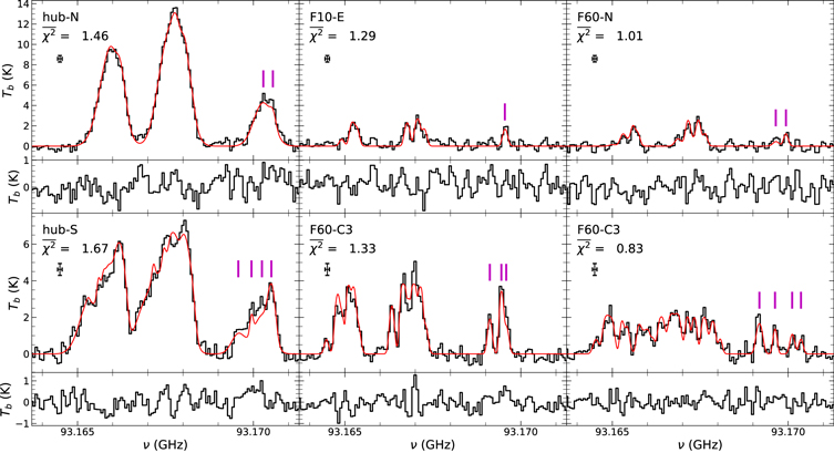
Figure 8. Observed spectrum (black histogram) with the spectral fit (red curve) and the residuals after subtracting the fit (immediately below the spectral plot) for a few selected pixels. The magenta bars indicate the frequency of the isolated hyperfine component (ν0 = 93.176252 GHz) shifted to the velocity components in the fit. The associated hubs/filaments of the pixels are indicated in the upper-left corner along with the  value for the fit. The cross with error bars indicates the rms uncertainty (σ = 0.32 K) in brightness temperature and the velocity channel width of
  .
.
Download figure:
Standard image High-resolution imageFurther inspection reveals a few limitations of our spectral models, mostly caused by oversimplified assumptions. Our spectral model assumes a single temperature for all velocity components along the line of sight, which is not valid in regions with significant internal heating, particularly in hub-N and hub-S. As a result, the  values are fairly large in both hubs (Figure 20). Note that we do not use spectral fits in hub-N or hub-S for later analysis. Meanwhile, we also assume a single beam-filling factor to reduce npar. This is not a good approximation in transition zones, where multiple velocity components are involved with varying emission fractions within one single beam. Because of the criterion for velocity separation between any two velocity components, the selection will favor single component with a larger line width in convergent regions of multiple velocity components.
4.4. Velocity Components Associated with Filaments
Once the kinematics are derived from spectral fitting, we then try to find velocity components associated with each individual filaments in the position–position–velocity (PPV) space. We apply the friends-of-friends (FoF) method, one of the widely used techniques to identify groups of galaxies in galaxy redshift surveys, initially presented by Huchra & Geller (1982). This method has recently been used to study filamentary cloud structures in molecular line observations (e.g., Hacar et al. 2013, 2018; Henshaw et al. 2014). The FoF is an algorithm used to establish membership in a group by identifying “friends” of an existent group member according to their linking lengths within predetermined thresholds. Such a linking length criterion results in a pairwise identification that is commutative. If member 1 finds member 2 a friend, member 2 also finds member 1 a friend. In the PPV space, the linking length is usually specified by the combination of projected separation and velocity difference. To start the process, one usually assigns a first member, the seed, of a group. The algorithm then searches for its “friends,” which are neighbors within predetermined thresholds for the linking length. After including the friends of the seed, the search continues iteratively to find and include friends of the newly identified members until no more friends can be found in the catalog. At this point, the members of the group are determined.
Given the limited sensitivity and spectral resolution, we simply search for relevant velocity components in each individual filament without further differentiating substructures in any filament. The thresholds are chosen to reflect the limitation of our observations. We consider a pair of PPV components to be friends if their angular separation is within half a beam and their velocity difference is less than two channels, i.e.,  . In addition, we set a boundary at the end point of the spine to separate filaments from the two prominent hubs; otherwise, all the filaments connected with a hub will become one single group. To identify PPV components associated with a filament, we assign pixels in the spine to be seeds and apply the FoF method to find members. Multiple seeds are assigned for a filament when regions have spectral fits that do not fully trace the spine. The derived PPV distribution and the components associated with each filament are shown in Figures 9 and 10 for Field-N and Field-S, respectively. Animations showing the PPV distribution rotating about a fixed position are available.
Figure 9. Selected views of position–position–velocity (PPV) distribution for the derived kinematics in Field-N. Blue dots are components associated with filament F10-E, while green dots are those associated with F60-N. Gray dots indicate velocity components in hub-N and unclassified structures. (a) Viewing from the south. (b) Viewing from the east at an angle nearly perpendicular to the velocity axis. A velocity gradient on parsec scale is clearly detected. More velocity components are present in hub-N than those in filaments. At 1.98 kpc, a structure of 1 pc long subtends an angular size of 104″. An animated version of this figure is available as a 3D flyby. The video duration is 15 s.
(An animation of this figure is available.)
Download figure:
Video Standard image High-resolution imageFigure 10. Selected views of position–position–velocity (PPV) distribution for the derived kinematics in Field-S. Blue dots are components associated with filament F60-C3, green dots with F60-S, and red dots with F60-C2. Gray dots indicate velocity components in hub-S and unclassified structures. (a) A view from the south. (b) A view from the southeast at an angle nearly perpendicular to the velocity axis. A velocity gradient on parsec scale in the filament F60-C3 is clearly detected. More velocity components are present in hub-S than those in filaments. At 1.98 kpc, a structure of 1 pc long subtends an angular size of 104″. An animated version of this figure is available as a 3D flyby. The video duration is 15 s.
(An animation of this figure is available.)
Download figure:
Video Standard image High-resolution imageWe also compare the derived kinematics with the averaged velocity plot of the isolated hyperfine component of the  emission along a given coordinate axis (Figures 11 and 12). In Field-N, a general velocity gradient is present mainly along the north–south direction so we average spectra along R.A. to examine the mean velocity pattern as a function of decl. (Figure 11(b)). The velocity of all the components in the PPV space is projected as a function of decl. (Figure 11(c)), where colors indicate components in different filaments. In Field-S, a general velocity gradient is roughly along east–west direction so spectra are averaged along the decl. axis (Figure 12(b)). The velocity of all the PPV components is projected as a function of R.A. (Figure 12(c)), where components associated with the three filaments are shown in three colors. In general, the derived velocity distribution agrees very well with the observed velocity pattern. A slow velocity gradient is present along several filaments, especially in filaments F10-E, F60-N, and F60-C3. Note that kinematics at the boundary between hub-S and filaments F60-C3 and F60-S are very complicated such that a perfect separation is not realistic.
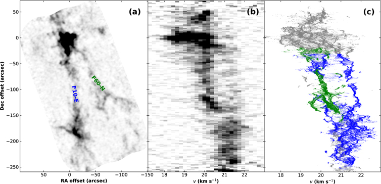
Figure 11. Gas kinematics as a function of decl. in Field-N. (a) Integrated intensity map of Field-N with labels for identified filaments. (b) Position–velocity plot of averaged spectra of the isolated component of the  emission as a function of decl. Spectra are averaged along the axis of R.A. (c) Similar position–velocity plot to (b) but for velocity determined in the hyperfine spectral fits. Blue points are velocity components associated with filament F10-E, and green points are associated with filament F60-N. Gray dots indicate velocity components in hub-N and unclassified structures.
Download figure:
Standard image High-resolution image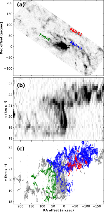
Figure 12. Gas kinematics as a function of R.A. in Field-S. (a) Integrated intensity map of Field-S with labels for identified filaments. (b) Position–velocity plot of averaged spectra of the isolated component of the  emission as a function of R.A. Spectra are averaged along the axis of decl. (c) Similar position–velocity plot to (b) but for velocity determined in the hyperfine spectral fits. Blue points are velocity components associated with filament F60-C3, green points with filament F60-S, and red points with F60-C2. Gray dots indicate velocity components in hub-S and unclassified structures.
Download figure:
Standard image High-resolution image4.5. Basic Properties of N2H+ Filaments
In general, the velocity gradient and dispersion along the filaments are better traced with the  line, which highlights the inner dense portion of the filaments better than the
  line does. This is likely due to the lower upper-level energy and higher critical density of
  . In addition,
  is known to quickly react with CO to form
  in outflow regions (Jørgensen et al. 2004; Lee et al. 2004; Busquet et al. 2011; Chen et al. 2011). Unlike
  , which may be excited by outflow shocks (Zhang et al. 1999),
  preferentially traces dense and quiescent gas.
Once the association with a filament is determined, we analyze the physical properties of a filament using data within 0.1 pc from its spine to avoid confusion from branches. The width of the mask is based on the angular resolution of the column density map (Lin et al. 2016) that has a lower spatial resolution of 0.1 pc. Because the  emission may have moderate optical depth and varying abundance compared to dust continuum emission, we estimate the mass in the filaments by linearly interpolating a column density map,
  , derived from the iterative SED analysis with a spatial resolution of 0.1 pc (Figure 2 in Lin et al. 2017). The filament total mass, M, is computed by integrating the column density within 0.1 pc from the spine. One important parameter for a filament is its linear mass, which is the total mass normalized by the filament length,
  . The linear mass of our observed filaments is in the range of 75–
 , with a mean value of
  (Table 2). In general, filaments in Field-N are more massive than filaments in Field-S.
Table 2. Physical Properties of Filaments
| Filament | Mℓ |

|
Nsub | αvir |

|

|

|
τa |
|---|---|---|---|---|---|---|---|---|
( ) ) |
( ) ) |
( ) ) |
( ) ) |
(Myr) | ||||
| Field-N | ||||||||
| F10-E | 105 ± 47 | 80 ± 30 | 1.625 | 1.2 ± 0.7 | 1.0 ± 0.6 | 0.5 ± 0.3 | (1.3 ± 0.9) × 10−4 | 1.8 |
| F60-N | 116 ± 52 | 64 ± 33 | 1.137 | 0.6 ± 0.4 | 0.9 ± 0.5 | 0.6 ± 0.2 | (1.3 ± 0.7) × 10−4 | 1.6 |
| Field-S | ||||||||
| F60-C3 | 84 ± 38 | 78 ± 26 | 1.529 | 1.4 ± 0.8 | 0.9 ± 0.7 | 0.4 ± 0.2 | (1.0 ± 0.7) × 10−4 | 2.7 |
| F60-S | 75 ± 34 | 88 ± 68 | 1.548 | 1.8 ± 1.6 | 1.1 ± 0.9 | 0.5 ± 0.5 | (0.7 ± 0.7) × 10−4 | 1.9 |
| F60-C2 | 78 ± 35 | 66 ± 44 | 1.201 | 1.0 ± 0.8 | 0.8 ± 0.5 | 0.3 ± 0.4 | (0.2 ± 0.3) × 10−4 | 3.6 |
Note.
aDepletion time if no mass replenishment.Download table as: ASCIITypeset image
4.6. Inflow Motion Along Filaments
The velocity profiles along individual filament spines are shown in Figure 13 with the origin starting at the end point closer to the hubs. Kinematics along the spines show highly structured filaments with multiple velocity components in many regions. Note that kinematics in filament F60-C3 are affected by hub-S (see Figure 6(b)) over a region between projected distance of 1.2–1.4 pc, where many pixels with four velocity components are present. On the basis of the complex structures in the PPV space (Figures 9 and 10), simple analyses along the spines will not be able to follow important and relevant structures in the filaments. Because we are interested in the collective effect of inflow motions along each filament, we approximate the filament by a cylindrical geometry and perform principal component analysis (PCA) to individual PPV distributions to determine the general orientation and velocity gradient of the filament. PCA is a statistical procedure widely used to describe the covariance structures of a set of variables and allows us to identify the principal directions in which the data vary. The principal components are found by calculating the eigenvectors and eigenvalues of the covariance matrix. The eigenvector with the largest eigenvalue, i.e., the first principal component, is the direction of greatest variation, where the scatter of the data from this axis is minimized. The amount of the total variance accounted for by the first principal component is assessed by its significance, which is equal to the percentage of the largest eigenvalue in the sum of all the eigenvalues. In our case, the first principal component is used to identify the general orientation of a filament and the velocity gradient along such axis. This is an approach similar to previous studies using linear regression, which requires velocity as a function of position, i.e., single velocity in one position (e.g., Kirk et al. 2013; Henshaw et al. 2014). Because multiple velocity components are present in our filaments, PCA allows a fit for general orientation and velocity gradient with the full ensemble of PPV components. The derived velocity gradient is in the range of  , with a mean value of
  (Table 2). The first principal component has significance higher than 96.6% in all filaments.
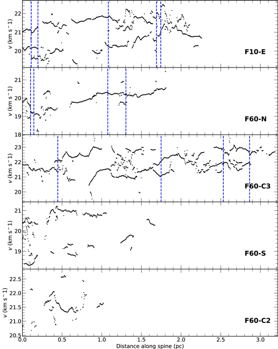
Figure 13. Velocity profiles along filament spines, starting from the end point closer to the hubs. The vertical dash lines mark the projected locations of the 3 mm dense cores (Ohashi et al. 2016) within 0.1 pc away from the spines. Hub-S and filament F60-C3 are contacted sideways over a region near distance ∼1.3 pc.
Download figure:
Standard image High-resolution image4.7. Transonic Turbulent Motions
In general, the line width of the  emission with higher angular resolution is narrower than that of the
  . Because
  tends to trace regions of higher densities, the inner part of the filaments may be less affected by radial collapse or turbulence of ambient gas onto filaments. We compute the nonthermal velocity dispersion, σnt, with

where Δυ is the observed line width, kB is the Boltzmann constant, Tg is the gas temperature, and  is the mass of
  . Because
  is of relatively high molecular weight, it is a good tracer to probe the nonthermal velocity dispersion. The sound speed in the gas is given by

where μ = 2.33 is the mean molecular weight, and mH is the mass of H. The ratio σnt/cs determines whether the gas motion is subsonic with σnt/cs ≤ 1, transonic with 1 < σnt/cs ≤ 3, or supersonic with σnt/cs > 3. This scheme is similar to the choice of transonic regime used by Arzoumanian et al. (2013). Figure 14 shows the distribution of the ratio σnt/cs for the entire mosaic regions. The two mosaic fields have similar distributions with a peak at σnt/cs ∼ 0.7 and a slow decay into transonic regime. Among all the positions with successful fits, 60% have subsonic nonthermal motions and 96% include subsonic and transonic motions altogether. Regions with supersonic motions account for only 4% of the whole population and are preferentially associated with the two hubs, which are main sites of active star formation. Still, the limited spectral resolution of  may cause confusion in the fitting algorithm to misidentify two subsonic components very close in velocity as one transonic component. The fraction of subsonic velocity components may be further increased if both angular and spectral resolutions improve in future studies. Within 0.1 pc along filament spines, σnt/cs is in the range of 0.8–1.1 with a mean value of 0.9, implying moderate transonic nonthermal motions (Table 2).
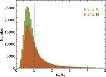
Figure 14. Histogram of all the positions as a function of nonthermal velocity dispersion normalized to local sound speed,  . The two fields show a similar distribution with a main peak that occurs at
  and a slow decay into transonic regime. The majority of the positions have nonthermal motions in the subsonic to transonic regimes.
Download figure:
Standard image High-resolution image5. Discussion
5.1. Mass Accretion Rates
Once the observed filament length, ℓobs, and the observed velocity gradient, ∇υobs, are measured, one can estimate the mass accretion rate by approximating a filament with a cylindrical geometry. The observed filament length and velocity gradient are both affected by the projection effect. We assume that a filament of mass M has an inclination angle, i, with respect to the line of sight. Following the method used by Kirk et al. (2013), one may express the observed quantities with the actual filament length, ℓ, and flow velocity υ along the filament as


where  . The mass accretion rate,
  , is then given by

In practice, it is impossible to identify a filament if it is inclined along the line of sight (i ∼ 0°) because it gives a null projected length. Observational bias is expected in estimates of mass accretion rate due to the projection effect. For example, a filament perfectly inclined on the plane of the sky (i ∼ 90°) will not have any detectable velocity gradient. Assuming a moderate inclination angle of i = 45°, we list in Table 2 the mass accretion rate,  , and the depletion time, τ, which is the timescale to exhaust all the mass in the filament by the measured accretion rate without mass replenishment from the surroundings. The accretion rates will vary in 73% if we assume a fluctuation of ±15°, i.e., 30°–60° inclination angles. To date, only a few observations have successfully detected inflow motion along filaments toward their converging hubs (e.g., Kirk et al. 2013; Lee et al. 2013; Peretto et al. 2013, 2014; Lu et al. 2018). Overall, the inflow motion along the filaments generates an observed velocity contrast, υobs, in the range of 0.4–
 . The flow velocity measured in IRDC G14.2 is in the range of 0.3–
 , which is comparable to previous studies if considering the variation in inclination.
Using the column density maps (Lin et al. 2016), we estimate the enclosed gas mass within FWHM to be  for both hub-N and hub-S. The measured core size (FWHM) is 0.25 pc for hub-N and 0.30 pc for hub-S. Assuming a spherical geometry, we obtain the mean number density of
  and
and  in hub-N and hub-S, respectively. These numbers are consistent with those reported by Busquet et al. (2016). The corresponding freefall time is
  in hub-N and 1.1 × 10⁵ yr in hub-S. The total mass accretion rate through the two filaments, F10-E and F60-N, connecting to hub-N is
  , which accumulates 22 M⊙ within one tff, about 20% of the mass in hub-N. Similarly, the two filaments, F60-C3 and F60-S, associated with hub-S deliver at a mass accretion rate of
  , which gathers 19 M⊙ within one tff, roughly 16% of the mass in hub-S. Because IRDC G14.2 is magnetized with a mean field strength of 0.35–0.55 mG, the contraction time is likely on a timescale 2–3 times longer than what is expected from a freefall collapse (Santos et al. 2016). Therefore, the filamentary accretion flow may account for nearly half of the mass in the hubs within one contraction timescale and is sufficient to alter the dynamical evolution of the hubs.
5.2. The Virial Parameter in  Filaments

The dynamical stability of a system is often assessed by the virial parameter, αvir. In the case of filaments, one compares the linear virial mass,  , to the observed linear mass, Mℓ. The gravitational instability of a pressure-confined isothermal gas layer with uniform magnetic fields has been studied by Nagai et al. (1998). In their models, the layer fragments into filaments, and a subsequent fragmentation to cores may occur in a filament if its linear mass is over a critical value
  . This model, however, does not include the nonthermal pressure support, which is important in massive star-forming regions. Following earlier studies (e.g., Fiege & Pudritz 2000; Arzoumanian et al. 2013), we apply the effective sound speed,
  , which combines the local thermal motions of interstellar molecules given by Equation (4) with nonthermal motions of the bulk of gas given by Equation (3). We estimate the virial mass per unit length with the mean effective sound speed,
  , of all the velocity components in a filament

The linear mass, Mℓ, however, is calculated from column density integrated along the line of sight without substructure details. To compare with the virial mass, we compute the mean linear mass accounted for substructures

where Nsub is the average number of substructures in the filament. We estimate this average number with  , where Nvel and Npix are the number of velocity components and the number of pixels in a filament, respectively. We then compute the virial parameter by comparing the virial mass to the mean linear mass accounted for substructures

The results are listed in Table 2. The value of  given by Equation (8) does not account for relative motion among substructures, whose contribution to pressure support remains unknown. Theoretical studies may provide useful insight. In addition, only the projected component of relative motion is observable. If substructures were to generate additional pressure support, the reported values of
  would be lower limits. The value of
  in the
  filaments is in the range of 0.6–1.8, with a mean value of 1.2, marginally virialized and likely to be in equilibrium. Our measured αvir range agrees well with the value range αvir = 0.7–2.0 obtained in the Orion Integral Filament (Hacar et al. 2018). Lower values of αvir are commonly observed in regions of high-mass star formation, as reported by Kauffmann et al. (2013) using a large complied sample of cloud fragments.
5.3. Comparison of Properties in Cores, Clumps, and Filaments
A comparison of the measured quantities in this work, such as the nonthermal velocity dispersion normalized to local sound speed, σnt/cs, and the virial parameter, αvir, is made with those reported in previous studies (Figure 15), including filaments identified in the  emission16
(magenta squares; Busquet et al. 2013), hubs and dense clumps identified in the 870 μm continuum emission (gray and green pentagons, respectively; Ohashi et al. 2016), and dense cores identified in the 3 mm continuum emission (blue diamonds; Ohashi et al. 2016). In this compiled sample, the size/length of the objects spans a range from 0.007 to 3.22 pc. Here, we consider the observed length of all the filaments to be lower limits of their actual lengths due to projection effects. The scale decreases from the
emission16
(magenta squares; Busquet et al. 2013), hubs and dense clumps identified in the 870 μm continuum emission (gray and green pentagons, respectively; Ohashi et al. 2016), and dense cores identified in the 3 mm continuum emission (blue diamonds; Ohashi et al. 2016). In this compiled sample, the size/length of the objects spans a range from 0.007 to 3.22 pc. Here, we consider the observed length of all the filaments to be lower limits of their actual lengths due to projection effects. The scale decreases from the  and
and  filaments, to the dense clumps, and then to the dense cores. We have also revised the measurements for the
  filaments (Busquet et al. 2013) using the updated distance of 1.98 kpc.
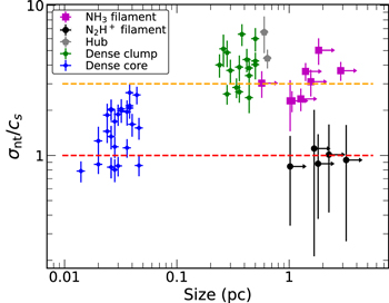
Figure 15. Nonthermal velocity dispersion normalized to local sound speed, σnt/cs, vs. size of cores/clumps and length of filaments in the compiled sample including cores, clumps, and filaments. Black dots indicate measurements of the  filaments in this work. The data for the
  filaments (magenta squares; Busquet et al. 2013), the 870 μm continuum hubs and clumps (gray and green pentagons, respectively; Ohashi et al. 2016), and the 3mm continuum cores (blue diamonds; Ohashi et al. 2016) are also shown. The upper limits of the subsonic (
 ) and transonic (σnt/cs = 3) regimes are indicated by red and orange dashed lines, respectively. The
  filaments show supersonic nonthermal motions, while the inner part of filaments traced by
  are mildly transonic. Dense clumps have stronger nonthermal motions than do dense cores.
Download figure:
Standard image High-resolution imageOverall, the  emissions in filaments show moderate transonic nonthermal gas motions (black dots, Figure 15), similar to what has been observed in other filaments (e.g., Hacar et al. 2013, 2018; Lu et al. 2018). The nonthermal motions observed in the dense clumps and
  filaments tend to be supersonic, with
  , while subsonic/transonic nonthermal motions (σnt/cs ∼ 1) are found in the dense cores and
  filaments (Figure 15). Compared to the mostly supersonic
  emission, the inner volume of the filaments with higher gas density shows weaker nonthermal motions, i.e., smaller σnt. Transonic filaments have been observed and are likely to be dynamically decoupled from the large-scale turbulent fields (Hacar et al. 2013, 2016; Chen et al. 2016). Meanwhile, the compact 3 mm dense cores also have weaker nonthermal motions compared to the more extended dense clumps, a phenomenon that has also been reported by Sanhueza et al. (2017) and Lu et al. (2018). There are a few implications of this weaker nonthermal support toward smaller scales. Naively, a virialized system under self-gravitation is expected to show an increasing pressure support near the central region, which is the opposite of the trend in σnt/cs in our sample. In the case of spherical geometry (clumps and cores), such reduced nonthermal support at small scales may be a feature of global hierarchical collapse (Naranjo-Romero et al. 2015) or an outcome of dissipation of turbulence giving a transition to coherence (Goodman et al. 1998, 2009; Pineda et al. 2010; Gong & Ostriker 2011; Chen et al. 2018). Nevertheless, an increasing support of magnetic fields that compensates the nonthermal pressure also cannot be ruled out (Kauffmann et al. 2013). Numerical simulations of prestellar cores based on the hierarchical collapse scenario develop structures not in hydrostatic equilibrium but with smaller infall velocities in the inner part, giving a smaller σnt/cs (Naranjo-Romero et al. 2015). The largest velocities occur in the outer parts of the core, making the collapse outside-in. On the other hand, dissipation of turbulence due to a reduction of field-neutral coupling at higher density can also produce weaker nonthermal motions at small scales, rendering a pressure difference that may initiate a pressure-driven inflow to allow mass accretion toward the central part of the system (Myers & Lazarian 1998). Whether these mechanisms also operate in filaments will need more theoretical investigation.
In Figure 16, we compare the gas mass, M, to the virial mass, Mvir, in cores and clumps (Ohashi et al. 2016) as well as the mean linear mass,  , to the linear virial mass,
  , in filaments (this work and Busquet et al. 2013). Sources that appear below the boundary line of αvir = 1 (red dash line) are expected to be gravitationally bound. In our sample, the
  filaments have significantly higher linear virial mass due to their supersonic nature. The nonthermal motions in the
  filaments are mildly transonic. Similar to the
  filaments, the dense clumps are also in equilibrium. Dense cores, the smallest scales in our sample, are gravitationally bound with significantly lower values of αvir < 1.
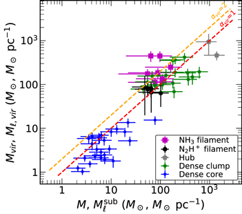
Figure 16. Comparison between the virial mass, Mvir, for cores/clumps and linear virial mass,  , for filaments with the observed gas mass, M, or mean linear mass,
  , in IRDC G14.2. The ratio of virial mass to gas mass gives the virial parameter, αvir. The slopes corresponding to
  (red dash line) and αvir = 2 (orange dash line) are also shown. Objects with αvir < 1 are gravitationally bound.
Download figure:
Standard image High-resolution image5.4. Uncertainties in Mass Estimates
A few factors may contribute to uncertainties in the mass estimates in our sample. We calculate uncertainties for derived quantities by propagating errors in dependent variables. The uncertainty in the distance measurement of IRDC G14.2 is roughly 7% (Xu et al. 2011), which affects all the quantities involving physical scales and masses derived from flux measurements. Following the discussion by Sanhueza et al. (2017), we adopt uncertainties of 28% and 23% for the dust opacity and gas-to-dust mass ratio. The uncertainties in the dust temperature and column density measurements with the iterative SED fits (Lin et al. 2016) are around 20% and 10%, respectively. Hence, the uncertainty in the gas linear mass after propagating all the errors is roughly 45%. The uncertainties in the virial mass estimates arise from the dispersion in the effective sound speed,  , and are listed in Table 2. The uncertainty in the ammonia temperature measurements applied to the
  filaments, dense clumps, and dense cores are assumed to be 3 K, which is a more conservative estimate. The absolute flux measurements of ALMA Band 3 is good within 5% (Section 2), so the typical uncertainty in mass estimates of dense cores is around 48%. Regarding mass estimates for
  filaments, the uncertainty in the ammonia abundance,
  , is assumed to be 67% on the basis of the dispersion in the
  abundance studies in IRDCs (Pillai et al. 2006). In the current analyses, we ignore uncertainties caused by plausible biases in identifying cores, clumps, and filaments. Such uncertainty may require simulations to obtain a fair estimate.
5.5. Dynamical Stability and Virial Parameters
We further investigate the dependence in the virial parameter, αvir, with physical scales, s, and nonthermal velocity dispersion normalized to local sound speed, σnt/cs. A decreasing trend in αvir with decreasing scales, from  filaments to
  filaments, then to dense clumps, and down to dense cores, can be discerned (Figure 17(a)). To investigate whether this decreasing trend is robust, we perform linear regression for a bootstrapping statistical sample of 50,000 synthetic data sets. Care has been taken to ensure sufficient sample size for convergence. We then calculate the mean and standard deviation of the slopes and intercepts derived from the sample. This analysis is necessary because of the unknown inclination angle of the filaments. For cores and clumps, we assume normal distribution of uncertainty in physical scale (diameter), s, and virial parameter, αvir. In the case of filaments, the uncertainty in αvir is assumed to be a normal distribution. Because of the unknown intrinsic length of a filament, we assume a uniform distribution of inclination angles and allow the deprojected length to reach a given maximum length, ℓmax. We vary ℓmax to examine how the slope and intercept depend on ℓmax. Our test finds a weak dependence that
  for maximum intrinsic filament length in the range of ℓmax = 5–8 pc (black line in Figure 17(a)). The slope decreases monotonically to 0.22 for longer intrinsic filament lengths up to 20 pc. The αvir also shows a decreasing trend with σnt/cs. We perform similar bootstrapping statistical analysis with a normal distribution for all the uncertainties and obtain
  (black line in Figure 17(b)).
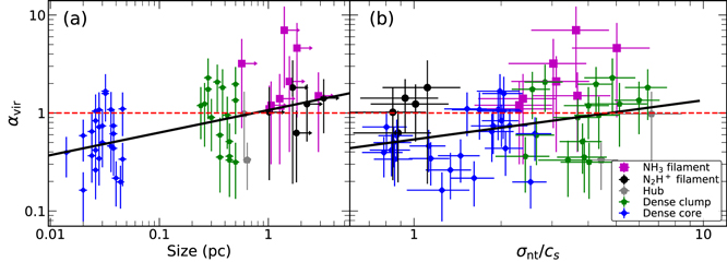
Figure 17. (a) Virial parameter, αvir, as a function of the size, s, of the observed objects. Red dash line indicates αvir = 1. The decreasing trend in αvir with decreasing scale persists as previously reported by Ohashi et al. (2016). Linear regression derived from the bootstrapping statistical samples gives  (black line). (b) The virial parameter, αvir, as a function of nonthermal velocity dispersion normalized to local sound speed,
  . Filaments show slightly higher αvir than cores and clumps. A decreasing trend in αvir with decreasing σnt/cs is seen, suggesting that objects with smaller σnt/cs tend to be more dominated by gravity. Linear regression renders
  (black line).
Download figure:
Standard image High-resolution imageThe  filaments added in this work are consistent with such behavior in
  previously reported by Ohashi et al. (2016, Figure 17(a)). Because lower αvir indicates a condition of gravity dominating over the pressure support, this decreasing trend suggests an increasingly important role of gravity at small scales. Meanwhile, αvir also shows a general decreasing trend with decreasing nonthermal motions, σnt/cs (Figure 17(b)), suggesting that objects with smaller σnt/cs tend to be more dominated by gravity. As also shown in Figure 15, the nonthermal motions are supersonic in the
  filaments and dense clumps and transonic in the
  filaments and dense cores. In general, filaments show a slightly higher
  compared to dense clumps and cores. The
  filaments and dense clumps have αvir ∼ 1, likely to be in equilibrium, while dense cores, though transonic, are gravitationally bound with αvir < 1.
Our current analyses of αvir in the cores and clumps do not include magnetic fields, which are expected to provide additional support against self-gravity (Van Loo et al. 2014) and increase the value of αvir. The magnetic field strength in IRDC G14.2 reported by Santos et al. (2016) is in the range 0.32–0.55 mG, corresponding to the Alfvén Mach number in the range of  . For a magnetized cloud with uniform density distribution, the virial mass is given by (Lu et al. 2015)

where  is the virial mass for a nonmagnetized sphere. Hence, the magnetic fields in IRDC G14.2 are able to increase the nonmagnetized virial mass, Mvir, by a factor of 1.8–3.0, which is not necessarily negligible. However, because the field strength was measured in a much larger scale, it is not clear how αvir will vary at scales of our filaments and cores. Meanwhile, an inflow toward a hub will drain the mass in a filament unless mass replenishment occurs to sustain the filament. If filaments are long-lasting features, mass replenishment is needed and will most likely come from the surroundings. Striation features around filaments are thought to be related to this accretion scenario (e.g., Palmeirim et al. 2013). Observationally, such a radial collapse has been reported only in a filament in Serpens South (Kirk et al. 2013). The velocity gradients along filaments observed in IRDC G14.2 may drain the filaments and induce mass replenishment from the surroundings, perhaps a radial accretion onto the filaments, producing external ram pressure that helps to keep the filaments bound.
5.6. Massive Star Formation Scenarios
A few theoretical scenarios have been proposed to explain massive star formation. In the turbulent core model (McKee & Tan 2002), massive stars form via a monolithic collapse of a massive core, which is approximately in hydrostatic equilibrium with pressure support from turbulence. Additional feedback from low-mass protostars such as radiative heating also help to suppress fragmentation in massive cores. Hence, cores forming massive stars usually harbor one or a few stars (Krumholz et al. 2007). Alternatively, scenarios allowing continuous mass accretion through the protostellar phase have also been developed. The competitive accretion model (Bonnell et al. 2001) describes the accretion in clusters as a dynamical phenomena. A cloud first fragments into cores of thermal Jeans mass and forms a cluster of low-mass protostars. Subsequent Bondi–Hoyle type accretion of surrounding gas in the parent clump allows protostars to grow in mass. Those protostars located near the center of the cluster accrete gas of higher densities and gain mass faster, having a better chance to become massive stars. Recently, the global hierarchical collapse model (Vázquez-Semadeni et al. 2009; Ballesteros-Paredes et al. 2011; Hartmann et al. 2012) advocates a picture of molecular clouds in a state of hierarchical and chaotic gravitational collapse, in which local centers of collapse develop throughout the cloud while the cloud itself is contracting. The collapse applies to all scales but not necessarily starts at precisely the same instant. In this scenario, a small number of stars may form early throughout the cloud before global contraction increases the gas density and the bulk of stellar population is formed in the center. This model has reproduced quantitatively a few observational properties of star-forming clusters, such as high local star formation rates with low global efficiencies (Vázquez-Semadeni et al. 2009) and the age spreads in young cluster members (Hartmann et al. 2012).
To date, a good range of surveys has been conducted in the IRDC G14.2. A star-forming scenario that can explain the main observational results is gradually emerging. Young stellar populations observed in the X-ray and infrared wavebands reveal a significant deficit of high-mass YSOs (Povich et al. 2009, 2016; Povich & Whitney 2010). This absence of massive stars in the intermediate stage of cluster formation has been reproduced in simulation involving global hierarchical collapse (Vázquez-Semadeni et al. 2017). In the millimeter waveband, clumps and cores have been identified to study core mass function (Busquet et al. 2016; Ohashi et al. 2016). Both prestellar and protostellar cores are gravitationally bound with low values of virial parameter αvir < 1. None of the prestellar and protostellar cores is more massive than 22 M⊙, suggesting that cores do not acquire all their mass before forming a protostar but continuously gain mass through protostellar phase. In contrast with forming a few protostars via a monolithic collapse of a massive core, the dense cores in IRDC G14.2 are likely accreting from the surroundings that are fed by their parent clumps or filaments (Gómez & Vázquez-Semadeni 2014). In the current study, we find that protostars and cores are preferentially located in the hubs and filaments. The filaments deliver mass to the hubs with sufficiently high accretion rates to affect the hub dynamics within one freefall time (∼105 yr). These observational features are consistent with the global hierarchical collapse scenario if IRDC G14.2 produces massive protostars later in time and matures with the Salpeter IMF.
5.7. Alternative Dynamical Interpretation and Substructures in Filaments
The unknown inclination introduces an unavoidable bias in identifying a filament and a fairly large uncertainty in the estimates of the accretion rate along the axis. It has also rendered two plausible scenarios, inflow or expansion, for the observed velocity gradients as discussed in the case of IRDC G035.39−00.33 (Henshaw et al. 2014). If filaments are in expansion, higher pressure and stronger nonthermal motions will be expected in hubs and filaments. The substructures in the  filaments show subsonic nonthermal motions (Figure 14). Both the hubs and
  filaments are gravitationally bound (Figure 16). Hence, the expansion scenario seems less favorable in IRDC G14.2.
Recent studies of filaments have shown the presence of substructures, i.e., fibers, that collectively form a filament (Li & Goldsmith 2012; Hacar et al. 2013, 2018; Sokolov et al. 2017). These substructures have also been reproduced in numerical simulations and are important to our understanding of filament formation mechanisms (Smith et al. 2014, 2016; Moeckel & Burkert 2015; Clarke et al. 2017). It is not yet clear whether fibers are long-lived, preexisting structures or density perturbations developed during accretion from an inhomogeneous turbulent medium. The internal kinematics among fibers may also affect the dynamical stability of a filament. With the limited sensitivity and velocity resolution of  in our current observations, we notice multiple velocity components present in roughly 1/3 of our spectra but cannot trace and differentiate individual fibers reliably. Although weak emission is detected in the total intensity maps, we were not able to obtain successful fits. This produces disconnected short segments in one seemingly coherent structure in the PPV space. In addition, a small number of velocity components are present between fibers. It is not clear whether all these components may be neglected by assuming their spectra resulted from line blending of components in the neighboring fibers. This issue occurs in every filament but is particularly severe for filaments in Field-S. Future observations with improved spatial and spectral resolution will be needed if each individual fibers are to be robustly identified.
6. Conclusion
We have performed full-synthesis imaging to map the  emission in the IRDC G14.2 with two mosaic fields that cover hub-N and hub-S as well as their associated filaments using the ALMA 12 m Array, the ACA, and the TP array. Our observations resolve the filaments with resolutions of ∼0.034 pc. Kinematics are derived from a sophisticated spectral fitting algorithm that accounts for line blending, large optical depth, and multiple velocity components. Our main findings are as follows:
- 1.We identify five filaments with the dense, quiescent gas tracer using the FilFinder package. Embedded YSOs and dense cores are preferentially associated with hubs and filaments. Large-scale velocity gradients are detected, suggestive of accretion flows toward the two dominant hubs, where protoclusters are located. In general, filaments show mildly transonic nonthermal motions, and ∼1/3 of the positions show multiple velocity components.
- 2.PCA is used to find the dominant flow direction and velocity gradient in each filament. Assuming a moderate inclination angle of i = 45°, mass accretion rates along filaments are in the range of. Simple estimates show that the accretion by filaments is significant to affect the dynamics of hubs within one freefall time (∼105 yr).
- 3.The emission profiles are analyzed with the RadFil package for measuring the width of the filaments. The width ranges from 0.05 to 0.09, with a mean value of 0.07 pc, which is smaller than but comparable to the universal 0.1 pc width reported by previous Herschel studies.
- 4.Our filaments are marginally virialized and likely to be in equilibrium with a mean value of αvir ∼ 1.2. Magnetic fields may play a role to provide additional support in filaments with small αvir.
- 5.A comparison study of measured in the filament, filament, dense clumps, and 3 mm dense cores is made. The filaments and dense clumps show supersonic nonthermal motions, while the filaments and dense cores are mostly subsonic and transonic. The decreasing trend in αvir with decreasing scales persists, suggesting an increasingly important role of gravity at small scales. We also found that αvir decreases with decreasing nonthermal motions. The large-scale filamentary accretion flows are likely feeding hubs, which harbor dense small-scale structures. In combination with the absence of high-mass protostars and massive cores, our observational results are consistent with the global hierarchical collapse scenario.




We are indebted to a careful anonymous referee, who helped significantly to improve the paper. This work is supported by the Taiwan Ministry of Science and Technology, project Nos. MOST 106-2119-M-007-022-MY3 and MOST 105-2119-M-007-022-MY3. G.B. is supported by the MINECO (Spain) grants Nos. AYA2014-57369-C3 and AYA2017-84390-C2-2-R. P.S. was financially supported by Grant-in-Aid for Scientific Research (KAKENHI No. 18H01259) of Japan Society for the Promotion of Science (JSPS). A.P. acknowledges financial support from grant No. UNAM-PAPIIT IN113119, México. This paper makes use of the following ALMA data: ADS/JAO.ALMA#2013.1.00312.S, #2015.1.00418.S. ALMA is a partnership of ESO (representing its member states), NSF (USA), and NINS (Japan), together with NRC (Canada), MOST and ASIAA (Taiwan), and KASI (Republic of Korea), in cooperation with the Republic of Chile. The Joint ALMA Observatory is operated by ESO, AUI/NRAO, and NAOJ.
Facility: ALMA. -
Software: CASA (McMullin et al. 2007), MIRIAD (Sault et al. 1995), FilFinder (Koch & Rosolowsky 2015), RadFil (Zucker et al. 2018b), TOPCAT (Taylor 2005),
Appendix A: N2H+ (1−0) Velocity Channel Maps
Here we present the velocity channel maps of the isolated  component of the
  emission with velocity step of
  for Field-N (Figure 18) and Field-S (Figure 19).
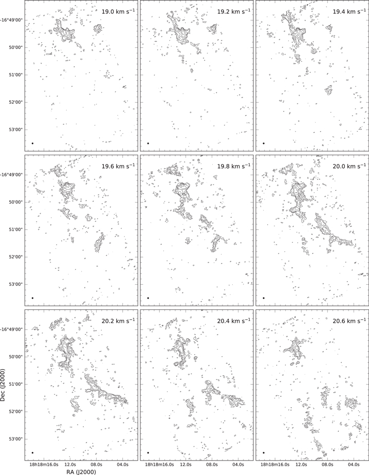
Figure 18.
Velocity channel maps in the Field-N. Contour levels are 0.08, 0.13, 0.21, 0.34, 0.54, and  with a beam size of 3
48. (The complete figure set (4 images) is available.)
Download figure:
Standard image High-resolution image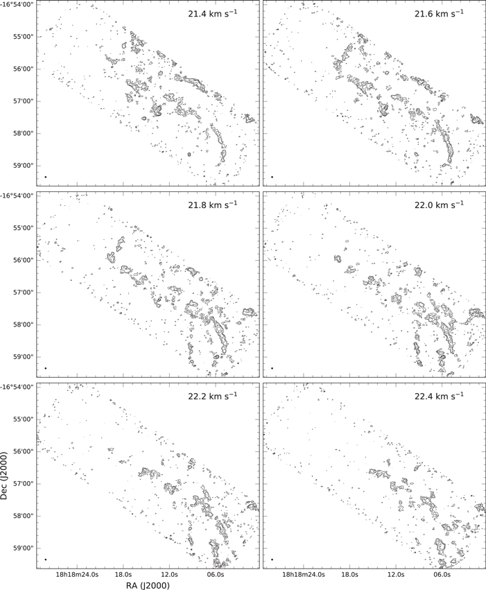
Figure 19.
Velocity channel maps in the Field-S. Contour levels are 0.07, 0.11, 0.16, 0.25, 0.39, and  with a beam size of 3
15. (The complete figure set (5 images) is available.)
Download figure:
Standard image High-resolution imageAppendix B: N2H+ Spectral Models and the Fitting Procedure
The fitting procedure in the current work uses an improved algorithm to handle a large amount of spectral data on the basis of our previous studies (Chen et al. 2010, 2011). In a low-temperature environment, the radiation of cosmic microwave background at  may not be negligible. One can find the intensity of line emission and continuum emission of a cloud to be

where  is the Planck function at a temperature Tbg, Sν is the source function determined by the gas in the cloud, and
  and
and  are the respective optical depth of the line and continuum. Assuming that the gas along the line of sight is isothermal at a gas temperature of Tg, one can approximate the source function by
  . In observations, the intensity of line emission is obtained after subtracting the continuum emission

In terms of brightness temperature, one finds

where  . The emission at a given velocity is described by three parameters, the velocity υi, the column density Ni, and the FWHM as line width Δυi. The optical depth of Nhfc hyperfine components of the
  emission is computed with
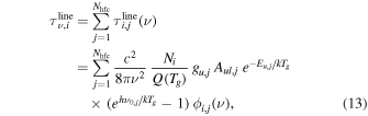
where the subscript denotes the jth hyperfine component,  is the rest frequency,
  is the statistical weight of the upper level,
  is the spontaneous emission rate of the transition, and
  is the upper-level energy. Values of these quantities are obtained from the Splatalogue database in National Astronomical Radio Observatory (NRAO). For J = 1−0 transition, there are Nhfc = 7 hyperfine components. The line profile ϕi,j(ν) is given by
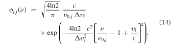
Therefore, the optical depth of the line emission including all the velocity components in Equation (12) is

where ϒ is the number of velocity components in the model spectrum. Furthermore, the observed brightness temperature, Tb, may be reduced by a beam-filling factor, fb. Assuming a single filling factor for all velocity components, our model spectrum is described by

Note that the beam-filling factor is coupled with the attenuation caused by the continuum optical depth, i.e.,  , in our model fitting algorithm.
Given ϒ velocity components along one line of sight (one pixel), we optimize the model spectrum with  parameters for minimization of the reduced χ2 value,
  , using the Levenberg-Marquardt method. The reduced
  value is normalized to the degrees of freedom, ndof

where ndata is the number of data points, and  is the number of fitted parameters. For our image cubes, a maximum of four velocity components, ϒmax = 4, is sufficient to produce reasonable fits. To avoid underestimating emission of very narrow line width, refinement of each channel into 11 uniformly divided subchannels in frequency is performed. In each frequency channel, the mean value of
  in all the subchannels is used to compare with the observed value.
Initial guesses of velocity components are identified from the cross-correlation function between the observed spectrum and a template spectrum with a narrow line width of  . For spectra with many velocity components, the cross-correlation function may not always deliver the best guess, so we allow a maximum of six velocity components to serve the initial selection set. To determine how many velocity components are needed to fit an observed spectrum, an optimizer simply scans through all the combinations made out of the six most probable velocity components. The combinations of ϒ selection out of six components are given by
 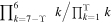 . Therefore, the maximum number of all the available combinations for an initial set of six will be 56. Each combination of initial guess is optimized for a solution, and the corresponding reduced χ2 value,
  is computed. Only pixels with more than nine channels above 3σ level are processed. A solution with any velocity component of spectral peak lower than 2σ is excluded from the final selection. We also require separation between any two velocity components to be larger than two channels, i.e.,
  , to avoid excessive overmodeling. The solution that gives the minimum value of
  among all the selected combinations is used to represent the kinematics of the working pixel. Note that only bright spectra of multiple peaks, such as pixels in hubs, are actually processed for all the 56 combinations of initial guess. After processing the entire cube, we further reject components of spectral peak lower than 3.5σ to avoid poorly constrained components. This rejection is similar to the criterion in previous studies (e.g., Kirk et al. 2013; Hacar et al. 2018). Although this methodology requires more computation time, it does not require visual inspection in intermediate steps and likely produces a uniform, less biased interpretation of a large data cube.
For IRDC G14.2, we have successfully derived the kinematics for 149,410 and 199,336 pixels in Field-N and Field-S, respectively. Figure 20 shows the spatial distributions of  rendered from our fitting algorithm, and Figure 21 shows the corresponding histograms. Overall, pixels in the central regions of the hubs tend to have the largest
  values. This is mostly caused by our oversimplified assumptions leading to Equation (16). For example, a temperature gradient is likely to occur in these internally heated hubs with multiple embedded YSOs. In addition, the beam-filling factor, fb, may not necessarily be a constant for all the velocity components along the line of sight.
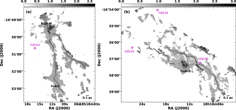
Figure 20. (a) Reduced χ2,  , distribution of 149,410 pixels in Field-N. (b) Same distribution of 199,336 pixels in Field-S.
Download figure:
Standard image High-resolution image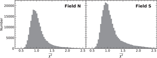
Figure 21. Histogram of  in Field-N (left) and Field-S (right). The
  distribution peaks around ∼0.95 with a weak tail toward large value, which occurs in the hubs and the margin of the fields.
Download figure:
Standard image High-resolution imageFootnotes
- 14
FilFinder is available at https://github.com/e-koch/FilFinder.
- 15
RadFil available at https://github.com/catherinezucker/radfil.
- 16
The
data have lower spatial resolution (82 × 7
) than do the data. We set for the observed filaments, which do not differentiate substructures.


