Abstract
We present the largest and most homogeneous collection of near-infrared (NIR) spectra of Type Ia supernovae (SNe Ia): 339 spectra of 98 individual SNe obtained as part of the Carnegie Supernova Project-II. These spectra, obtained with the FIRE spectrograph on the 6.5 m Magellan Baade telescope, have a spectral range of 0.8–2.5 μm. Using this sample, we explore the NIR spectral diversity of SNe Ia and construct a template of spectral time series as a function of the light-curve-shape parameter, color stretch sBV. Principal component analysis is applied to characterize the diversity of the spectral features and reduce data dimensionality to a smaller subspace. Gaussian process regression is then used to model the subspace dependence on phase and light-curve shape and the associated uncertainty. Our template is able to predict spectral variations that are correlated with sBV, such as the hallmark NIR features: Mg ii at early times and the H-band break after peak. Using this template reduces the systematic uncertainties in K-corrections by ∼90% compared to those from the Hsiao template. These uncertainties, defined as the mean K-correction differences computed with the color-matched template and observed spectra, are on the level of 4 × 10⁻⁴ mag on average. This template can serve as the baseline spectral energy distribution for light-curve fitters and can identify peculiar spectral features that might point to compelling physics. The results presented here will substantially improve future SN Ia cosmological experiments, for both nearby and distant samples.
Original content from this work may be used under the terms of the Creative Commons Attribution 4.0 licence. Any further distribution of this work must maintain attribution to the author(s) and the title of the work, journal citation and DOI.
1. Introduction
Type Ia (SNe Ia) provide excellent luminosity distances thanks to their empirically standardizable properties, such as the correlations between the intrinsic peak luminosity and the light-curve shape (Pskovskii 1977; Phillips 1993), as well as the color (Tripp 1998). The comparison of the high-redshift SNe Ia with the low-redshift sample led to the first evidence for cosmic acceleration (Hamuy et al. 1996; Riess et al. 1998; Perlmutter et al. 1999). By mapping out the expansion history of the universe, SNe Ia have become an essential tool for understanding the nature of dark energy (e.g., Riess et al. 2007; Suzuki et al. 2012; Scolnic et al. 2018; Brout et al. 2022).
The precision of SN Ia cosmology is now limited by systematic errors that cannot be reduced by simply observing more SNe. These include uncertainties introduced by photometric calibration, evolutionary effects, host-galaxy environment, and uncertain extinction laws. Observations in the near-infrared (NIR) offer a promising direction to achieve more accurate results for cosmology (e.g., Barone-Nugent et al. 2012; Burns et al. 2018; Stanishev et al. 2018; Avelino et al. 2019; Jones et al. 2022) with several advantages compared to the optical.
The NIR region is less affected by dust extinction, minimizing the reliance on uncertain dust laws (e.g., Cardelli et al. 1989; Krisciunas et al. 2000; Johansson et al. 2021). The bias toward low-reddening objects in high-redshift observations is also minimized in the NIR, reducing the systematic differences between the colors of low- and high-redshift SN Ia samples. Furthermore, both theory (Kasen 2006) and observations (Krisciunas et al. 2004; Wood-Vasey et al. 2008; Mandel et al. 2009; Folatelli et al. 2010; Kattner et al. 2012) have shown that SNe Ia have more uniform peak luminosities in the NIR. Therefore, smaller light-curve-shape correction is needed to standardize normal SNe Ia in the NIR (e.g., Krisciunas et al. 2004; Dhawan et al. 2018; Galbany et al. 2022), which could reduce the systematic errors caused by potential evolutionary effects.
Due to the lack of sufficient NIR data, the majority of the empirical light-curve fitters currently available for SN cosmology rely on optical data only and have not yet included NIR coverage. The only three light-curve models that cover NIR so far are SuperNovae in object-oriented Python (SNooPy; Burns et al. 2011, 2014), the hierarchical Bayesian SED Model for SNe Ia (BayeSN; Mandel et al. 2009, 2011, 2022), and SALT3-NIR (Pierel et al. 2022).
K-corrections are necessary to allow for the comparison of rest-frame magnitudes of objects at various redshifts (Oke & Sandage 1968). Several efforts have been made to improve the accuracy of the K-corrections for SNe Ia, such as the utilization of the cross-filter K-corrections for high-redshift SNe Ia (Kim et al. 1996) and the construction of time-series spectral templates (Nugent et al. 2002; Hsiao et al. 2007) of the spectral energy distribution (SED). Uncertainties in the K-corrections, caused by intrinsic variations in the broadband colors and spectral features, directly affect the error budget of the distance measurements (e.g., Hsiao et al. 2007; Boldt et al.2014).
As the next generation of space telescopes such as the James Webb Space Telescope and the Nancy Grace Roman Space Telescope (RST) look further to the red, an accurate description of how the SN Ia SED varies in the NIR is important for a wide range of applications. It is particularly crucial for any NIR SN Ia dark energy experiments, whether explicit K-correction calculations are needed or not. For example, in the case of SALT3 (Kenworthy et al. 2021), an accurate underlying SED model is required to evade K-correction calculation. However, current NIR spectral templates have room for improvements. For example, the NIR region of the spectral template of Hsiao et al. (2007) and Hsiao (2009) is only based on 52 NIR spectra of 30 SNe Ia compiled by Marion et al. (2009), a sample too small to adequately capture intrinsic variations. Further complicating the matter, the features in the regions of strong telluric absorptions are completely obscured due to its narrow range of redshifts in this sample.
As in the optical, the NIR spectral features of SNe Ia are highly correlated with the light-curve shape, the primary parameter (Hsiao 2009). The correlation is especially evident in the H-band break (e.g., Hsiao et al. 2013; Ashall et al. 2019a, 2019b), the most prominent SN Ia spectral feature in the NIR (Kirshner et al. 1973; Wheeler et al. 1998). This suggests that the SEDs can be accurately predicted given only the light-curve shape (Hsiao et al. 2007; Hsiao 2009). Characterizing the NIR spectroscopic diversity of SNe Ia became one of the main motivations for the second stage of the Carnegie Supernova Project (CSP-II; Hsiao et al. 2019; Phillips et al. 2019).
CSP recognizes the potential of NIR observations and contributed high-precision observations of hundreds of SNe Ia over the past roughly two decades. The first phase of CSP (CSP-I; 2004–2009; Hamuy et al. 2006) aimed to construct a data set of both optical and NIR light curves in well-understood and calibrated photometric systems (Contreras et al. 2010; Stritzinger et al. 2011; Krisciunas et al. 2017) with telescopes located at Las Campanas Observatory. A separate high-redshift (0.1 < z < 0.7) component of the project produced an NIR Hubble diagram in the rest-frame i band and examined the potential of shifting SN Ia cosmology toward the red (Freedman et al. 2009).
CSP-II (2011–2015) focused on building the low-redshift optical and NIR anchor with an unbiased sample of SNe Ia in the smooth Hubble flow (Phillips et al. 2019). A second component of the project aimed to obtain a statistically significant sample of NIR spectra (Hsiao et al. 2019) for SNe of all types (e.g., Davis et al. 2019; Shahbandeh et al. 2022). In collaboration with the Harvard–Smithsonian Center for Astrophysics Supernova Group, a large sample was mainly acquired using the then newly commissioned Folded-port InfraRed Echellette (FIRE; Simcoe et al. 2013) mounted on the Magellan Baade telescope. Over the course of the CSP-II campaign, 620 NIR spectra of 149 SNe Ia were obtained.
The CSP-II sample is much larger than those in previous works (roughly an order of magnitude increase), and most observations are accompanied by accurate photometry. The vast majority of the SNe Ia have time-series NIR spectroscopic observations and complementary photometry, such that the phases of the spectra and the light-curve-shape parameters of the SNe Ia can be accurately determined. Another key improvement is in the regions of strong telluric absorption. The high throughput of FIRE, in combination with the large aperture of Baade, provided an adequate signal to recover the SN flux in the telluric regions for most of our spectra. Using this data set, we construct NIR time-series spectral templates as a function of phase and light-curve-shape parameter.
In this paper, we present the NIR spectra obtained by the CSP-II and a new set of NIR spectral templates constructed using this data set. Section 2 describes the selection criteria and characteristics of the sample used. In Section 3, the methodology of the template construction is described in detail. The properties of the template and its impact on cosmology are discussed in Section 4. Finally, a summary is presented in Section 5. In this work, unless noted otherwise, the phase is relative to the time of the rest-frame B-band light-curve maximum.
2. Sample
In this section, we describe the data set used in this work. The sample of NIR spectra comes entirely from the CSP-II (Hsiao et al. 2019; Phillips et al. 2019). Approximately three-quarters of SN Ia spectra were obtained using FIRE in the high-throughput prism mode. In contrast with the majority of other NIR spectrographs, this configuration of FIRE consistently provides an adequate signal in the regions of heavy telluric absorption to enable telluric corrections. Using the Pα P-Cygni feature in our sample of type II SN (SN II) spectra, the telluric corrections were shown to recover the feature to 10% precision or better in 70% of our sample (Davis et al. 2019). The conventional notion that features in the telluric regions can only be obtained by space-based or airborne observatories is no longer correct.
The features in the telluric regions are crucial, as they will inevitably be shifted into observed filters when we study SNe Ia at a range of redshifts. This was the main difficulty in obtaining accurate NIR K-correction uncertainties in past studies (e.g., Boldt et al. 2014). For this reason, as well as to ensure the homogeneity of the data set, we opted to only include FIRE spectra taken in the prism mode 31 for this work. This amounts to an initial sample of 461 NIR spectra of 142 SNe Ia, which we narrowed through the selection criteria described below. The spectra observed in FIRE prism mode have an approximate wavelength coverage from 0.8–2.5 μm, and resolutions of R ∼ 500, 450, and 300 in the J, H, and K bands, respectively. Details of the observations and data reduction can be found in Hsiao et al. (2019).
2.1. Selection Criteria
With the goal of constructing spectral templates as a function of the color-stretch parameter (sBV ; Burns et al. 2014) and phase, the following selection criteria were applied in this order:
- 1.
- 2.Each SN must have a reliable time of the B-band maximum (
 ), and each spectrum must have a phase that is less than or equal to 100 days. This step further excludes 83 spectra of 30 SNe Ia.
 - 3.Each spectrum was visually inspected for significant host-galaxy contamination by comparing with spectra in a similar parameter space. This final step further excludes eight spectra of four SNe.

Out of the initial 461 spectra of 142 SNe, 331 spectra of 94 SNe Ia remain after the three-step sample cut. Figure 1 illustrates the change of sample size after applying each selection criterion. All spectra that passed through the first two steps, 339 spectra of 98 SNe, are available in the CSP website. 32 A log of these spectra is listed in Appendix A.
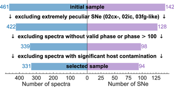
Figure 1. The number of spectra and SNe Ia as each selection criterion is applied.
Download figure:
Standard image High-resolution image
 and the sBV
of the sample SNe were obtained by fitting multiband CSP light curves using SNooPy with max_model. An arbitrary cutoff phase was set at 100 days relative to the B-band maximum, well past the phase range relevant for light-curve fitting.
and the sBV
of the sample SNe were obtained by fitting multiband CSP light curves using SNooPy with max_model. An arbitrary cutoff phase was set at 100 days relative to the B-band maximum, well past the phase range relevant for light-curve fitting.
The peculiar SNe Ia were identified based on their light curves and optical spectra. Note that spectra of the slow-declining 91T-like (Filippenko et al. 1992a; Phillips et al. 1992) and fast-declining 91bg-like (Filippenko et al. 1992b; Leibundgut et al. 1993) SNe Ia were kept in the sample intentionally for the following reasons: (1) Their NIR spectral features, while extreme, were shown to extend the properties of normal SNe Ia (e.g., Hoeflich et al. 2002; Hsiao et al. 2015; Phillips et al. 2022). (2) Studies have shown that 91bg-like and fast-declining SNe Ia in general are standardizable and do not impact Hubble constant measurements significantly (e.g., Burns et al. 2014; Hoogendam et al. 2022; Phillips et al. 2022; Yang et al. 2022). (3) The inclusion of these SNe will help broaden the sBV baseline since they are on the edges of the distribution.
Only eight spectra show significant host contamination. These are usually SNe Ia situated close to the host-galaxy core and taken at late phases when the background flux is comparable to or higher than the SN itself. The effects are shallow spectral slope and more diluted spectral features especially toward the red end. These were easy to identify through visual inspection and comparison to other spectra at similar phases. They also showed up as outliers during the dimensionality reduction step (Section 3.2) if there were included.
2.2. Sample Characteristics
The final sample of spectra that passed the selection criteria (331 spectra of 94 SNe) cover a wide range of heliocentric redshift, sBV , and phase (see Figure 2). A full range in sBV and phase is desirable as the goal here is to build a set of spectral templates as a function of sBV and phase. A wide range in redshift is also useful as spectral features are shifted out of regions that are heavily affected by telluric absorption. The sample SNe cover a heliocentric redshift range of 0.003 ≤ z ≤ 0.087 with a median of 0.021 and a color-stretch range of 0.48 ≤ sBV ≤ 1.30 with a median of 0.97. The r-band absolute magnitudes of the host galaxies are obtained using the Z-PEG (Le Borgne & Rocca-Volmerange 2002) SED software following the procedure described in Uddin et al.(2017).
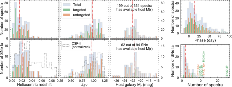
Figure 2. Characteristics of the selected sample of NIR spectra. The top panels present the distributions of spectra in redshift, sBV , host-galaxy r-band absolute magnitude, and phase; the bottom panels show the distributions of SNe in redshift, sBV , host-galaxy r-band absolute magnitude, as well as the number of spectra per SN. The green and orange distributions represent SNe discovered by targeted and untargeted surveys, respectively. The median value of each total distribution is indicated with a vertical dashed–dotted line. For comparison, the distributions (normalized to peak) of the full CSP-II SNe Ia sample from Phillips et al. (2019) are plotted with dashed lines in the lower panels.
Download figure:
Standard image High-resolution imageThe majority of the SNe Ia (70%) in this sample were discovered by untargeted searches. This is the result of the survey strategy of CSP-II, designed to avoid bias toward bright and large host galaxies (Phillips et al. 2019). As shown in the bottom panels of Figure 2, SNe from untargeted searches extend out to higher redshifts and cover a wider range of the host-galaxy absolute magnitude compared to those from targeted searches. They also have a similar distribution in sBV except for a possible excess at the bright and slowly declining end. The normalized distributions of the full CSP-II SNe Ia sample (combined “Physics” and “Cosmology” samples from Phillips et al. 2019) are also shown in Figure 2. The selected sample for the template is representative of the full CSP-II sample in terms of sBV .
Next, we examine the distribution of the sample spectra and SNe in phase−sBV space (see Figure 3). Unsurprisingly, most spectra were taken near maximum light and belong to normal-bright SNe Ia. The sample spectra have a median sBV of 0.98 and a median phase of 14 days. Figure 3 then identifies the data that would provide the most improvement for the next iteration of template building: NIR spectra of fast-declining SNe in general, particularly at late phases. These observations are naturally difficult as these SNe are rare, intrinsically faint, and fade more rapidly than normal-bright SNe.
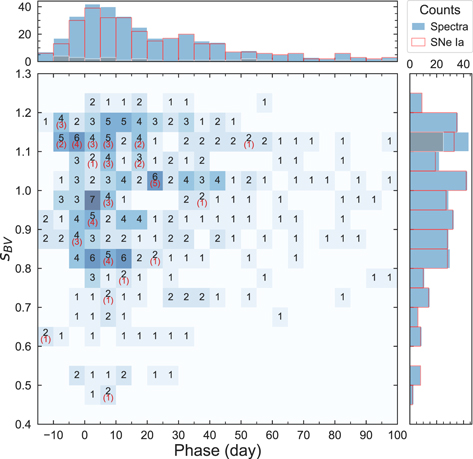
Figure 3. Two-dimensional histogram of the spectra/SNe in (phase, sBV ) with marginal distributions. The bin size is 5 days for phase and 0.05 for sBV . Each non-empty bin has a black label to show the number of spectra, with an additional red label beneath indicating the number of SNe if there are more than one spectrum that belongs to the same SN. The gray filled distribution represents the most well-sampled SN 2012fr in the selected data set.
Download figure:
Standard image High-resolution imageOur approach is to model the dependence of spectroscopic properties on phase and sBV as a hypersurface in the phase−sBV space (Section 3.3). The dearth of data in certain regions and the over-reliance on individual well-observed SNe (e.g., SN 2012fr has 25 spectra in the sample) may produce potential biases if the data represent the extremes in the respective bins. The best way to improve this is a larger sample that fills in the phase−sBV space. To characterize this potential bias, we compare the templates built with and without the 25 spectra of SN 2012fr in Section 4.1.
2.3. Spectrophotometric Accuracy
Since there are no spectrophotometric standard stars in the NIR that can be observed by FIRE, flux calibration was done using telluric standards (Hsiao et al. 2019). Each standard is an A-type main-sequence star similar to Vega (A0 V star) observed at a similar airmass, usually immediately before or after the science observation. The flux calibration is performed simultaneously with the telluric correction given the B and V magnitudes of the A0 V star, following the procedures outlined by Vacca et al. (2003). Here, we examine the spectrophotometric accuracy of our sample NIR spectra calibrated using this method in terms of the relative colors. Note that the vast majority of the spectra were observed at parallactic angle to prevent the change of spectroscopic colors caused by the slit loss.
To assess the spectrophotometric accuracy after flux calibration, the synthetic broadband Y − J and J − H colors measured directly from the spectra are compared to those from the corresponding light curves. All spectra were corrected for Milky Way (MW) extinction using the Schlafly & Finkbeiner (2011) dust map and the Fitzpatrick (1999) law assuming RV = 3.1. Spectroscopic colors were then measured from synthetic photometry using YJH filters. Due to the design of CSP-II, the photometric coverage has typically nightly cadence in the optical but has large gaps in the NIR (Phillips et al. 2019). Here, we took advantage of the simultaneous optical-to-NIR light-curve fitting of SNooPy, using the SNooPy models to interpolate the sparse data in the NIR. The MW extinction-corrected Y − J and J − H colors interpolated to the dates of the spectroscopic observations were then taken as the comparison photometric colors.
The comparison between the observed spectroscopic and photometric colors is shown in Figure 4. The rms of the difference between spectroscopic and photometric colors is around 0.2 mag in both Y − J and J − H, with the mean systematic difference within 0.1 mag. Furthermore, Hsiao et al. (2019) showed that the median color differences between 13 NIR spectra and well-sampled light curves are 0.08 mag in Y − J and 0.03 mag in J − H. This indicates that the spectrophotometric accuracy of this sample of NIR spectra (without the contribution of the interpolation uncertainty) is roughly at the 10%–20% level.
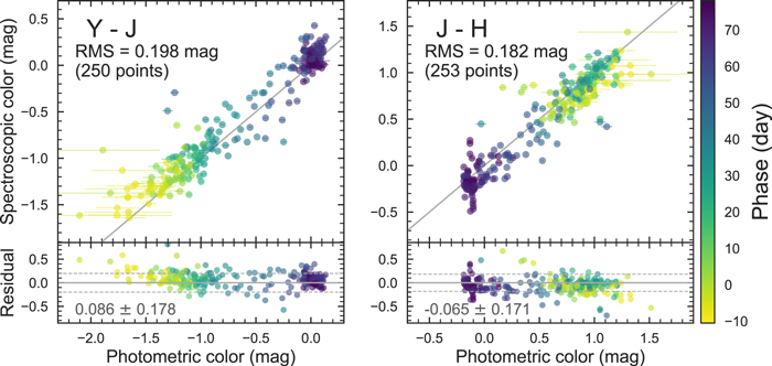
Figure 4. Comparison between the observed spectroscopic and photometric colors for the selected sample, color-coded by phase. Both are corrected for MW extinction. The solid lines in the top panels correspond to the ideal one-to-one correlations. The resulting rms is approximately 0.2 mag in both Y − J and J − H, and represents the upper bound in the spectrophotometric uncertainty, as this figure includes the uncertainty in the light-curve interpolation. In the bottom panels, the horizontal solid and dashed lines represent the mean and the dispersion of the residuals, respectively, with the values printed in the lower-left corner.
Download figure:
Standard image High-resolution imageAnother way to examine the spectroscopic colors is to look at their evolution over time. Figure 5 shows the resulting time evolution of the spectroscopic Y − J and J − H colors. There is clear evidence that the color evolution depends heavily on the sBV parameter, indicating that the spectroscopic colors are accurate enough to preserve such a signal. To avoid incurring further uncertainty from the interpolation of sparse data and the narrower phase coverage of SNooPy, we chose not to match the spectroscopic colors to the photometric colors in this work.
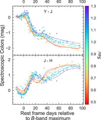
Figure 5. Time evolution of the sample spectroscopic colors in rest frame. The spectra were corrected for MW extinctions. The points are color-coded by the sBV of the SNe. To aid the visualization, Gaussian process regression (GPR) fits of the phase and sBV dependence are plotted as solid curves. The flux calibration of the spectra is accurate enough to preserve these correlations.
Download figure:
Standard image High-resolution image3. Methods
The goal of this work is to empirically construct a set of NIR spectral templates of SNe Ia based on observed data. The templates aim to quantify the following spectral properties: the time evolution, the correlation with a light-curve-shape parameter, and the remaining diversity in the form of statistical flux uncertainties. A summary of the procedure is outlined here, and the details are given below.
- 1.The spectra that satisfy the selection criteria are organized onto a common rest-frame wavelength grid (Section 3.1).
- 2.
- 3.
The final result can be used to reconstruct the normalized SN Ia SED, as well as the associated uncertainties, given the phase and the light-curve shape of a SN Ia. The focus of building the template was placed on the spectral features, since in SN Ia cosmological studies, the broadband colors can be corrected by matching photometric colors but the spectral features cannot.
Alternatively, we also explored a neural network approach using a conditional variational autoencoder (cVAE). The cVAE approach is able to produce promising results similar to those from the PCA+GPR method while being more flexible; see Appendix B for a discussion of the advantages and disadvantages of this proposed method.
3.1. Data Preparation
As the entire data set is observed with a single instrument and configuration by design, it is possible to create a common rest-frame wavelength grid that is representative of the pixel grid and can minimize the interpolation uncertainties. First, an average wavelength grid is determined by taking the mean calibrated wavelength of the sample spectra at each pixel in the observer frame. This wavelength grid was then de-redshifted by the median redshift of the sample (zmedian = 0.021). Finally, the sampling frequency of the grid was doubled by adding a mid-point between neighboring points, forming a rest-frame wavelength grid with 3673 wavelength points. The resulting wavelength interval ranges from ∼3 Å in the Y band to ∼9 Å in the K band.
All sample spectra were de-redshifted to the rest frame and corrected for MW extinction using the Schlafly & Finkbeiner (2011) dust map and the Fitzpatrick (1999) law assuming RV = 3.1. They were then interpolated onto the common wavelength grid described above. Note that, to prevent spurious flux values from dominating the PCA, sigma-clipping was performed before the interpolation, removing all flux values 5σ above or below the local mean with an average window size of 100 Å.
If PCA is performed directly on the observed spectra covering so wide of a wavelength range as the NIR, the principal components (PCs) would be dominated by regions of relatively high intrinsic flux (e.g., the z and Y bands) and spurious variations (e.g., the telluric regions and at the edges of the spectra). The model SEDs need to include the more subtle variations of the spectral features. To achieve this, dimensionality reduction was performed in seven wavelength regions. The wavelength regions were somewhat arbitrarily defined but designed to correspond to the zYJHK 33 filters with some overlap. The overlapping region ranges from ∼90 Å between W1 and W2 to ∼370 Å between W6 and W7, with roughly 50 sampling points in each. The seven wavelength regions are presented graphically in the top panel of Figure 6 and tabulated in Table 1.
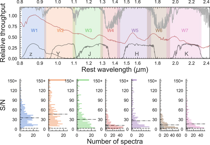
Figure 6. Top panel: definition of the wavelength regions. W1, W2, W3, W5, and W7 roughly correspond to the zYJHK filters (dark-gray solid curves), respectively, while W4 and W6 correspond to regions of strong atmosphere telluric absorptions (light-gray lines on top; de-redshifted by the median redshift of the SNe sample z = 0.021). A spectrum of SN 2012fr at +13 days past B-band maximum (red line) is plotted for illustration. Bottom panels: the distribution of the signal-to-noise ratio (S/N) of each wavelength region. The dashed–dotted horizontal lines mark the median S/N. The dashed horizontal lines mark the selection criterion of S/N ≥ 3. The gray stacked distributions in W4 and W6 represent the spectra that have poor telluric corrections. The gray stacked distribution in W7 (K band) indicates the spectra with spurious flux at the edge.
Download figure:
Standard image High-resolution imageTable 1. Wavelength Regions for Dimensionality Reduction
| Region | Filter a | λstart | λend | Median | Sample b | NPC c |
|---|---|---|---|---|---|---|
| (μm) | (μm) | S/N | Counts | |||
| W1 | z | 0.8100 | 0.9328 | 35 | 331 | 11 |
| W2 | Y | 0.9240 | 1.1072 | 47 | 331 | 11 |
| W3 | J | 1.0925 | 1.3041 | 31 | 327 | 10 |
| W4 d | ⋯ | 1.2865 | 1.4423 | 14 | 220 | 5 |
| W5 | H | 1.4198 | 1.7314 | 27 | 328 | 10 |
| W6 d | ⋯ | 1.6931 | 1.9361 | 16 | 238 | 6 |
| W7 | K | 1.8989 | 2.3300 | 20 | 291 | 8 |
Notes.
a Corresponding filter overlapping the most with the defined wavelength region. b Number of spectra after additional selection in each region; see Section 3.1. c Number of PCs kept for template construction; see Section 3.4. d Regions of strong telluric absorptions.Download table as: ASCIITypeset image
Additional selection criteria were imposed on the sample spectra in each wavelength region:
- 1.Each spectrum must have a median signal-to-noise ratio (S/N) ≥ 3.
- 2.In the telluric regions, W4 and W6, spectra that are over- or under-corrected for telluric absorptions were excluded by visual inspection.
- 3.In region W7 (K band), spectra with spurious flux values at the edge of the detector were excluded by visual inspection.
Separating a spectrum into wavelength regions has the added benefit that if the spectrum, for example, has poor telluric corrections, we do not have to discard other wavelength regions containing useful information. Approximately two-thirds of the sample have reliable telluric corrections, consistent with what we found in our SN II sample using the Paα feature (Davis et al. 2019).
The distributions of the S/N in each region are presented in the lower panels of Figure 6, and the final sample count and median S/N in each wavelength region are tabulated in Table 1. The S/N is highest in the Y band and decreases toward the blue and the red. As expected, the lowest sample count and S/N are found in the telluric regions, W4 and W6, with the median S/N staying above 10.
3.2. Dimensionality Reduction
An SN Ia spectrum contains a large number of elements, but they do not vary independently. Spectral variations are largely captured by only a few parameters (e.g., Nugent et al. 1995). It is thus possible to drastically reduce the dimensionality of SN Ia spectroscopic data, and PCA was chosen as the statistical technique for this purpose. It is widely used for modeling the SN spectra (e.g., Hsiao et al. 2007; Davis et al. 2019; Shahbandeh et al. 2022). PCA produces an orthogonal set of eigenvectors or PCs ranked by their eigenvalues, which give a measure of the amount of data variation they capture. In this work, the matrix diagonalization was done using the Python package scikit-learn (Pedregosa et al. 2011).
As mentioned in Section 3.1, the data were separated into wavelength regions in order to capture subtle variations. In each wavelength region, flux elements were placed on a uniform wavelength grid and normalized to have the same integrated flux in the region before PCA. Our chosen light-curve parameter is the color-stretch parameter sBV , since Δm15(B) and SALT x1 do not reliably classify fast decliners (Burns et al. 2014). The PCA operation has no knowledge of the phase and sBV labels for each spectrum nor the wavelength value for each flux element.
The resulting PCs are presented in Figure 7. Note that, in the figure, the PCs in the overlapped area between neighboring wavelength regions are not expected to be connected, since PCA is independently performed in each region. In regions W1–W6, it takes less than five PCs to capture >90% of the variations. Regions W2 and W3 (Y and J bands), in particular, only required two PCs each, indicating that the spectra are rather uniform. On the other hand, W7 (K band) requires six PCs to reach 90% of the variation, perhaps hinting at substantial diversity.
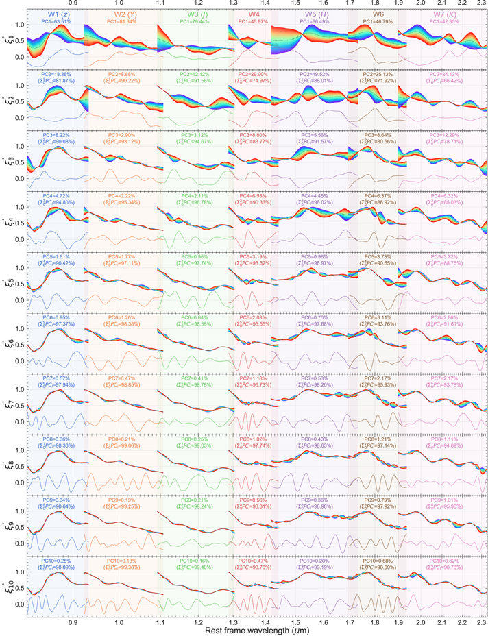
Figure 7. The first 10 PCs and the reconstructed spectra in each wavelength region. The PCs are ranked by the amount of data variation they describe (labeled on top of each panel in percent variation per PC and the cumulative percent variation). The solid curve on the bottom of each panel is the PC. The rainbow-colored curves are the PC-reconstructed spectra with 2σ variation on top of the mean (dashed curve).
Download figure:
Standard image High-resolution imageFigure 7 also shows the reconstructed spectra of 2σ variation on top of the mean spectrum. Familiar spectral features in the NIR then emerge, such as the Ca ii IR triplet in W1 (z band), Mg ii in W2 (Y band), the H-band break in W5 (H band), and Co ii in W7 (K band). Another example of the captured information can be found in PC1 and PC3 of W1 and W2, which appear to describe the strength and velocity of the spectral features, respectively, in both regions.
Each input spectrum can then be projected onto a PC in the multidimensional data space, providing an associated projection value. Mathematically, each input spectrum f m of n flux elements is then represented by the sum of all PCs ξ i weighted by the projections pi,m :

The projections are shown in Figure 8 with respect to phase and sBV . It is clear that the first several PCs in all regions have strong dependence on phase and sBV . The dependence is the weakest in the telluric regions W4 and W6 because of the lower S/N of the input data and the general lack of strong features. W5 (H band) shows particularly strong dependence in the top four PCs, giving confidence that the most prominent spectral features in the NIR can be well predicted with light curves alone. This offers the motivation for the next step: modeling the dependence of spectral properties, represented by the PC projections, as a hypersurface in phase-sBV space.
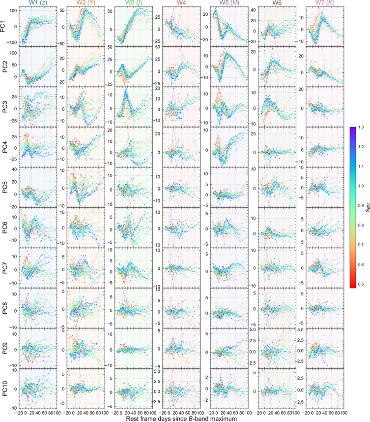
Figure 8. The projections of the input spectra onto the first 10 PCs. They are plotted with respect to the phase and color-coded using their sBV values. The solid lines connect the spectra of the same SN. In the higher-ranking PCs, the projections are highly correlated with phase and sBV in many PCs and wavelength regions, for example, PC2 and PC3 in W5 (H band) and PC1 and PC2 in W2 (Y band).
Download figure:
Standard image High-resolution image3.3. Modeling Parameter Dependence
In the previous step, the spectral data have been reduced in dimensionality such that each spectrum is represented by a few PC projections. Here, we will determine the dependence of the spectral properties on phase and sBV . The method chosen to map the projection hypersurface in phase-sBV space is GPR.
GPR has been shown to be successful at interpolating supernova light-curve data with intermittently missing data (e.g., Vincenzi et al. 2019; Pessi et al. 2022). The data characteristics are similar here (Figure 3). It also has the advantage of producing an uncertainty estimate to the hypersurface, which allows for the construction of not only the spectral templates but also the statistical flux uncertainties. In this work, GPR was performed using the Python package scikit-learn (Pedregosa et al. 2011). An example of the resulting hypersurface is shown in Figure 9, successfully capturing the spectral properties as a function of phase and sBV .
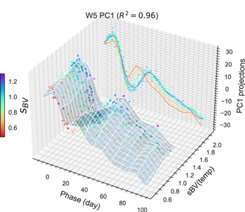
Figure 9. An example of the GPR mapping of the projection hypersurface in phase-sBV space. The side view of the hypersurface with various sBV slices is color-coded by sBV . Note that the side view of the data is the same as the one plotted in Figure 8. The R2 value noted on top of the figure is the coefficient of determination of the GPR prediction. The example shown is of PC1 in W5 (H band) and has one of the highest R2 values in our analysis.
Download figure:
Standard image High-resolution imageThe kernel setup for the GPR in this work was a constant kernel multiplied by a radial-basis function (RBF) kernel plus a white noise kernel. 34 The hyperparameters are optimized by maximizing the log-marginal likelihood. The details of the initial hyperparameter setting and optimal values can be found in Appendix C. Before performing GPR, the projection outliers were excluded by clipping spectra with projection values 5σ above or below the mean. The remaining projection values were then normalized to range from 0–1 to ensure consistency across all wavelength regions and PCs while maintaining a uniform kernel setup.
With the hypersurface in hand, one can obtain the modeled PC projection value and the associated uncertainties for each PC in each wavelength region, given the phase and sBV . Once it was decided which PCs are to be included, template spectra were then constructed via reverse transformation to return the projections to flux space. Finally, the spectra from individual wavelength regions were merged by matching the integrated flux in the overlapping regions and using the weighted average flux. 35 Now the question becomes: what is the minimum number of PCs necessary to describe the spectroscopic diversity and how to select them efficiently? This is addressed in Section 3.4.
An important feature of the new template is flux uncertainty estimation, indicating the confidence of the SED prediction. For example, the lack of data in certain parameter space translates to larger uncertainties in the template. The flux uncertainties were determined using procedures similar to the template spectra construction and a Monte Carlo approach. First, for each wavelength region and PC, the PC projection value was independently re-sampled 1000 times, assuming that the GPR hypersurface uncertainty has a Gaussian distribution. Crucially, we included all top 20 PCs for the uncertainty estimate, regardless of whether the PCs were included in the template construction. This is because those PCs not included in the template construction represent the observed SED variations that were not captured by the template. Each set of the re-sampled PC projections was then reverse transformed to the original flux space. The ratio of the template flux over the standard deviation of the re-sampled fluxes at each wavelength was then taken as the “S/N.” Finally, the S/Ns in the seven wavelength regions were merged by taking the weighted mean in the overlapping areas. An example of the template construction and the merging process can be found in Figure 10. Note that the choice of the number of iterations is based on the convergence of the median S/N.
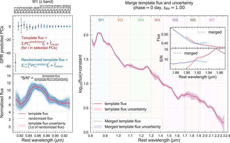
Figure 10. Example of the template construction in W1 (z band; left panel) and the merging process (right panel) of a maximum light spectrum of sBV = 1. In each wavelength region, the template flux is constructed by inverse-transforming the selected PCs (marked with filled red circles in the top-left example plot) that are predicted by GPR; and the template uncertainty is represented by the standard deviation of the inverse-transformed flux of 1000 sets of randomly sampled PCs assuming Gaussian error given the GPR prediction uncertainty. Then the template fluxes in neighboring regions are merged together by normalizing the integrated flux and taking the weighted flux in the overlapping region. The plotted example template in each region is normalized by the integrated flux in the overlapping area with the previous region. The flux uncertainties are connected together through taking the weighted mean S/N in the overlapping area. The inset in the right panel shows an example of such merging process between W6 and W7. The division of the seven wavelength regions is plotted in the background.
Download figure:
Standard image High-resolution imageThe PCA+GPR method we have presented here is robust, but has some limitations. First, it requires interpolations of the flux and their uncertainties onto a common wavelength grid prior to PCA. Second, PCA is a linear transformation and may require more dimensions to fully capture the variations in complex data distributions. Third, GPR results are sensitive to the kernel design (e.g., Stevance & Lee 2023). Furthermore, the dimension reduction and template generation parts do not communicate with each other, for example, one cannot improve the other iteratively. In Appendix B, we show that the neural network approach using cVAE can circumvent some of these drawbacks and achieve similar results. However, the spectral features in the telluric region are not well modeled with the cVAE approach compared with the current method.
3.4. Strategies for Selecting PCs
We considered three strategies for selecting the PCs for template construction:
- 1.Use the first N PCs and keep N fixed for all wavelength regions.
- 2.Use the first N PCs that capture a total variance that exceeds a fixed threshold in each wavelength region.
- 3.Use only the PCs with GPR coefficient of determination (R2) scores that exceed a fixed threshold in each wavelength region.
The R2 measures how well the GPR hypersurface predicts the PC projections of sample spectra and is defined as follows:

where  is the PC projection of the ith spectrum;
  is the GPR predicted PC projection given the same phase and sBV
values of the ith spectrum; and
is the GPR predicted PC projection given the same phase and sBV
values of the ith spectrum; and  is the mean of the PC projections of the sample spectra. A larger R2 value means that the GPR hypersurface captures more of the data variance. A value of R2 approaching 0 means that the predictions are close to the mean of projections and largely independent of the parameters.
To compare the three strategies quantitatively, we utilized the χ2 test:

where  is the observed spectrum flux of the ith spectrum,
  is the predicted template spectrum flux given the same phase and sBV
values of the ith spectrum, and the observed flux errors were used as the uncertainties σi
. Note that the template uncertainties are not considered since they might be correlated with the observed flux uncertainties. Each
is the predicted template spectrum flux given the same phase and sBV
values of the ith spectrum, and the observed flux errors were used as the uncertainties σi
. Note that the template uncertainties are not considered since they might be correlated with the observed flux uncertainties. Each  used for the test was color-corrected to match the color of
  before the comparison. The degrees of freedom (dof) were taken as the number of flux points minus the number of PCs used. Excluding the spectra with poor telluric correction and spurious flux values at the K-band edge (see Section 3.1), 225 observed spectra among the sample were used for the χ2 test.
Each wavelength region requires a different number of PCs to reach a total variance threshold. For example, the telluric regions W4 and W6, as well as W7 (K band) require more PCs to capture 95% of the data variance than the other regions; see panel (a) of Figure 11. As expected, the GPR R2 scores are the highest for the top-ranking PCs, as shown in panel (b) of Figure 11. However, they are not ordered perfectly, revealing some lower-ranked PCs with strong dependence on phase and sBV . Note that the GPR R2 scores are generally lower in the telluric regions W4 and W6. While this result may be revealing real spectral behavior, it more likely points to the observational challenges in these regions.
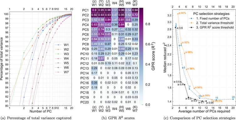
Figure 11. Panel (a): the cumulative total variance percentage of the first 20 PCs in each wavelength region. Panel (b): the heat map of the GPR scores of the first 20 PCs in each wavelength region, represented by the coefficient of determination (R2; which normally ranges from 0–1). Greater R2 means the GPR model captures more variance in the data set. Panel (c): comparison of three different strategies for PC selections in each wavelength region (see the text for details). The y-axis is the median χ2 per degree of freedom (dof) of the spectra sample, treating the template spectra as the expected value and the (number of points − number of PCs) as the dof. We adopt GPR score R2 ≥ 0.2 as our PC selection rule for template construction, as it efficiently reaches better χ2 per dof with fewer PCs compared to other strategies.
Download figure:
Standard image High-resolution imageThe performance of the three proposed PC selection strategies was then assessed via the χ2 test. In panel (c) of Figure 11, we plot the average number of PCs required across wavelength regions versus the median reduced χ2 for each strategy. Using a GPR R2 score threshold (strategy 3) shows a clear advantage over the other two strategies, as it requires fewer PCs in order to reach the same accuracy in the SED prediction. For example, to reach a reduced χ2 ∼ 1.43, the average number of PCs needed is 15 for strategy 1, 13 (total variance of ≥99.5%) for strategy 2, and eight (R2 ≥ 0.2) for strategy 3. This trend is consistent if we take the template uncertainties into consideration for the calculation, but the reduced χ2 values are consistently lower. Hence, we adopted strategy 3 with a threshold of R2 ≥ 0.2. The number of PCs used in each region is listed in Table 1. The GPR hyperparameters of the selected PCs are all converged to the optimal values, except the RBF length scale for sBV of PC1 in the W4 (telluric) region; see details in Appendix C. Note that even though some higher-ranked PCs are omitted when constructing the template flux, it is crucial to include these when estimating the uncertainties in the spectral template.
Having PC projections that are highly correlated with phase and sBV would be ideal for constructing spectral templates. However, spectral features with low GRP R2 scores could aid the search for a secondary parameter for improving SN Ia standardization or even point to interesting physics. For example, the early-phase NIR spectra of the transitional SN Ia iPTF13ebh have been shown to have strong C i features, most notably in the Y band (Hsiao et al. 2015). These spectra also have the most extreme PC projection values compared with other spectra at early phases, such as PC2, PC6, PC7, PC8, and PC10 in W2 (Y band; see Figure 8).
4. Results
Following the methodology set forth in Section 3, the NIR spectral templates of SNe Ia and corresponding statistical uncertainties can be constructed as a function of phase and the light-curve parameter sBV using PCA+GPR. In this section, we present the resulting NIR spectral templates and check how well they reproduce observed spectra. Here, we use K-corrections to assess the accuracies of the templates, even though they do not need to be explicitly calculated for spectrophotometric experiments or SED-based light-curve fitters.
The new NIR spectral template is available on the CSP website 36 and will be implemented in SNooPy (Burns et al. 2011), in where the NIR template can be attached to the optical region of the time-stretched (tstretched = t/sBV ) Hsiao template (Hsiao et al. 2007).
4.1. Spectral Templates
The template spectra constructed using the PCA + GPR method are able to replicate the spectral diversity in the sample spectra. In Figure 12, we highlight the spectral dependence on sBV in three wavelength regions and epochs: pre-maximum in the Y band, and post-maximum in the H and K bands.
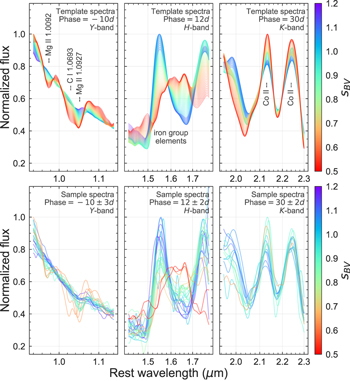
Figure 12. Comparisons between template (top panels) and observed spectra (bottom panels) for a range of light-curve color-stretch parameter sBV . The columns present the diversity for pre-maximum spectra around −10 days in the Y band (left), post-maximum spectra around 12 days in the H band (center), and post-maximum spectra around 30 days in the K band. In each panel, the spectra are normalized to have the same integrated flux in the wavelength region shown.
Download figure:
Standard image High-resolution imageThe left panels of Figure 12 present the pre-maximum spectra in the Y band at around −10 days. At these early phases, the photosphere arises in the outer and intermediate layers of the ejecta. Faster declining and fainter SNe clearly show stronger Mg ii λ 1.0092 and λ1.0927 μm features. The additional absorption feature on the blue wing of Mg ii λ1.0927 μm is captured by the template and appears to be only present in subluminous SNe Ia. This feature has been identified to be unburned C i λ1.0693 μm in several fast decliners: SN 1999by (Hoeflich et al. 2002), iPTF13ebh (Hsiao et al. 2015), SN 2012ij (Li et al. 2022), and SN 2015bp (Wyatt et al. 2021). An alternative identification of He i λ1.0830 μm has also been proposed in the context of the double-detonation scenario (Boyle et al. 2017).
At around two weeks past maximum, the prominent H-band break is at its peak strength (e.g., Hsiao et al. 2013). The template shows drastic differences in the profile shapes between slow and fast-declining SNe Ia (middle panels of Figure 12). These variations have been investigated in previous studies. The strength of the H-band break at its peak varies strongly with the light-curve decline rate (Hsiao et al. 2013, 2015). The velocity of the blue edge of the H-band break measures the 56Ni distribution and is also strongly correlated with sBV (Ashall et al. 2019a, 2019b). In the region between 1.6 and 1.7 μm, the spectral local minimum in a slow decliner is in contrast to a local emission feature in a fast decliner, which may be the result of a photosphere well within the central Ni-rich region (Hoeflich et al. 2002). Any viable explosion scenario needs to be able to explain these trends.
At approximately one month past maximum, the photosphere has receded to reveal the iron-peak elements in the inner layers. The K band is dominated by multiple lines of Co ii at this epoch (e.g., Gall et al. 2012). Interestingly, the template only shows a mild dependence of the feature shapes on the light-curve shape (right panels of Figure 12). The observed spectra show a range of feature strength but a weaker correlation with sBV compared to the H band. This perhaps points to a secondary parameter or contribution from a different spectral line that is not associated with the decay products of 56 Ni.
In Figure 13, we present the time-series comparison between our new template, the template of Hsiao et al. (2007) updated to include the NIR (Hsiao 2009), and the observed spectra within our sample. Note that the Hsiao template gives the average SED that is designed to match a stretch s = 1 SN Ia. For the Hsiao template, the variation with light-curve shape is accounted for through matching the time on the stretched time axis (tstretched = t/sBV ), assuming that a fast decliner also has a more rapid spectral evolution. Within the training sample, three well-observed SNe were selected for comparison: iPTF13ebh (sBV = 0.63) representing a fast decliner, SN 2013gy (sBV = 0.91) representing an average object, and SN 2013hh (sBV = 1.20) representing a slow decliner. As expected, the Hsiao template performs well when tasked to match an average SN Ia. On the other hand, the new template performs well for all sBV and shows a clear advantage at the extremes. This result demonstrates that the spectral feature dependence on the light-curve shape cannot be solely described by the speed of the evolution.
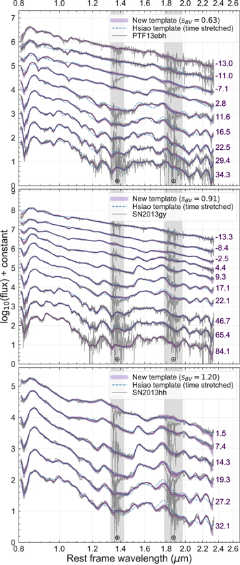
Figure 13. Comparison between template and observed spectra in the training sample. The panels show three well-observed time series from the FIRE sample: (top) sBV = 0.63, a fast decliner, (middle) sBV = 0.91, an average object, and (bottom) sBV = 1.20, a slow decliner. The new spectral template is shown by the solid colored curves with its 1σ uncertainty, while the Hsiao template is shown as blue dashed curves. All observed spectra were color-corrected to match the colors of the template spectra for presentation.
Download figure:
Standard image High-resolution imageIdeally, the performance of the new template should be assessed using an independent sample. In the left panel of Figure 14, the new and Hsiao templates are compared to the sample of Marion et al. (2009). Note that the phases relative to Vmax listed by Marion et al. (2009) were converted to phases relative to Bmax assuming that Vmax occurs 2 days after Bmax. Also note that Δm15(B) values were converted to sBV using Equation (4) of Burns et al. (2014). The sources of Δm15(B) values are tabulated in Table 2. Overall, the new template provides a better match than the Hsiao template especially for low and high sBV values, such as SN 2005am (sBV = 0.72). There are three notable disagreements for the NIR Ca ii triplet: SN 2003W at −6 days, SN 2004bv at −3 days, and SN 2001bf at 6 days. These could point to real diversity in the feature that is not captured by the template or observational artifacts near the short wavelength limit of the detector.
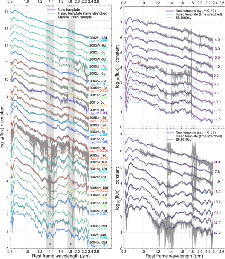
Figure 14. Comparison between template and observed spectra that were not included in the training sample. The new spectral template is shown by the solid colored curves with its 1σ uncertainty, while the Hsiao template is shown as blue dashed curves. The left panel shows comparisons with the sample of Marion et al. (2009), and the template is color-coded by sBV . The right panels show two subluminous SNe Ia from the literature: (top) SN 1999by (Hoeflich et al. 2002) with sBV = 0.63, and (bottom) SN 2015bp (Wyatt et al. 2021) with sBV = 0.67. All observed spectra were color-corrected to match the colors of the template spectra to focus on the spectral features.
Download figure:
Standard image High-resolution imageTable 2. List of SNe Ia Used for Spectral Comparison from the Sample of Marion et al. (2009)
| SN | z | Δm15(B) | Δm15(B) References | sBV a |
|---|---|---|---|---|
| (mag) | ||||
| 2000dk | 0.017 | 1.66 | Wang et al. (2019) | 0.70 |
| 2005am | 0.008 | 1.61 | Höflich et al. (2010) | 0.72 |
| 2000dm | 0.015 | 1.51 | Wang et al. (2019) | 0.77 |
| 2002 ha | 0.014 | 1.37 | Wang et al. (2019) | 0.83 |
| 2001br | 0.021 | 1.32 | Wang et al. (2019) | 0.85 |
| 2004ab | 0.006 | 1.27 | Chakradhari et al. (2018) | 0.88 |
| 2001en | 0.016 | 1.23 | Wang et al. (2019) | 0.90 |
| 2002cr | 0.010 | 1.19 | Wang et al. (2019) | 0.91 |
| 2002ef | 0.024 | 1.18 | Wang et al. (2019) | 0.92 |
| 2003cg | 0.004 | 1.17 | Wang et al. (2019) | 0.92 |
| 2003W | 0.020 | 1.15 | Wang et al. (2019) | 0.93 |
| 2001bg | 0.007 | 1.14 | Wang et al. (2019) | 0.94 |
| 2000dn | 0.032 | 1.13 | Wang et al. (2019) | 0.94 |
| 2002fk | 0.007 | 1.02 | Wang et al. (2019) | 0.99 |
| 2003du | 0.017 | 1.00 | Wang et al. (2019) | 1.00 |
| 2004bk | 0.023 | 0.98 | Wang et al. (2019) | 1.01 |
| 2004bv | 0.011 | 0.98 | Wang et al. (2019) | 1.01 |
| 2001fe | 0.014 | 0.96 | Wang et al. (2019) | 1.02 |
| 2001bf | 0.016 | 0.83 | Wang et al. (2019) | 1.08 |
| 2001dl | 0.021 | 0.80 | Marion et al. (2003) | 1.09 |
Note.
a Converted from Δm15(B) using Equation (4) of Burns et al. (2014).Download table as: ASCIITypeset image
As discussed in Section 2.2, the small number of NIR spectra of subluminous SNe Ia, especially at the late phase, is a limiting factor for the template at this particular phase space. Here, the template is compared to the spectra of two subluminous SNe from the literature: SN 1999by (sBV = 0.42; Hoeflich et al. 2002) and SN 2015bp (sBV = 0.67; Wyatt et al. 2021), shown in the right panel of Figure 14. These spectra were not included in our training sample. The spectra of SN 2015bp at various phases, including at more than 1 month past maximum, are well represented by the new template. This is despite the time gap of 50 days in the four FIRE spectra of SN 2015bp included in the training sample. Because of the limited range in the light-curve shape of our sample, reproducing the spectral features of SN 1999by with such a low sBV requires extrapolation on the hypersurface with GPR. Nevertheless, the spectral features of the template match exceptionally well to those of SN 1999by. Note especially that the C i features at early times were reproduced and are stronger than those of SN 2015bp. The Hsiao template simply fails at these low sBV values.
We also checked the broadband colors of the new template using the SNooPy model. The broadband colors of the new spectral template and the light-curve model of SNooPy are in general agreement within 0.2 mag for all colors and sBV values (Figure 15). The large discrepancies at the early phases may be due to the lack of observed data. The general agreement gives assurance that the merging of the seven wavelength regions at the last step of the template construction preserves the broadband color information. Note, however, that the spectral template should always be color-matched to the observed photometric colors of the SN Ia in question during the light-curve fitting process.
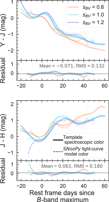
Figure 15. Comparison of the template spectroscopic colors (solid curves) and SNooPy light-curve model colors for various sBV values (dashed curves). The uncertainties on the SNooPy colors come from the uncertainties on the light-curve templates. In the bottom panels, the residuals are shown along with the mean (solid gray lines). The mean and rms values are also labeled.
Download figure:
Standard image High-resolution imageAnother test we did is to address the potential training bias toward SN 2012fr, the best-observed SN in the sample, with 25 spectra out of the total 331 sample spectra. Following the methodology of leave-one-out cross validation, we constructed another template without SN 2012fr following the same methodology to compare with the template built with the whole sample. The two templates were color-corrected to have matching broadband colors. The maximum flux difference is around 6% in the region near 0.85 μm, where SN 2012fr presents the detached high-velocity Ca ii feature at early times. In general, the differences between the two templates are negligible, with a median flux difference less than 1%.
4.2. K-correction Uncertainties
We utilized the definitions of K-correction uncertainties from Hsiao et al. (2007) to evaluate the performance of the new template. K-corrections obtained using the template spectra (Ktemp) were compared to those from observed spectra of our sample (Kobs) for different combinations of filters and redshifts.
The rms and the mean of the K-correction differences were then taken as the statistical and systematic uncertainties, respectively. The K-correction uncertainties were also compared to those computed using the Nugent (Nugent et al. 2002) and Hsiao (Hsiao et al. 2007) templates. The computations were done using the SNooPy package, while the template spectra were color-corrected to match the broadband YJH colors of the observed spectra before the computation.
Note that these uncertainty measurements were designed solely to evaluate how well the template can predict the spectral features of the observed spectra. The broadband colors of the template were corrected to match those of the observed spectra, as it is common practice in light-curve fitting to correct the template to the observed colors. These estimates do not include other effects, such as the uncertainty in the relative flux calibration discussed in Section 2.2.
In the most ideal case, one should assess the performance of the new template using a validation set of observed spectra that is completely independent of the template training set. In the NIR, the sample size is severely restricted by the telluric region, as discussed in Section 3.1. There is currently no spectral sample with reliable telluric regions besides the FIRE sample presented here, and after inspecting the telluric corrections, our sample was reduced by roughly one-third. Given this difficulty, we chose to evaluate its performance using a cross-validation technique described below.
First, a subsample with reliable telluric regions was chosen to form a “validation” pool. Next, we randomly selected 66 spectra from this pool to form the validation set, which constitutes 20% of the entire sample. The remaining 80% of the entire sample was then used as the training set. The training set was used to construct a template with the procedures outlined in Section 3, while the validation set was used to estimate the K-correction uncertainties. The process of splitting the sample, constructing the template, and estimating the K-correction uncertainties was repeated for 1000 iterations. The resulting uncertainty estimates converge rather quickly, generally after 50 iterations, while the 1000 iterations yielded Gaussian-like distributions.
Figure 16 presents the K-correction uncertainties as a function of redshift for several cases of single-filter K-corrections at low redshifts and cross-filter K-corrections at high redshifts. The mean and standard deviation of the 1000 iterations are shown as the solid curves and shaded regions, respectively. The observer-frame filters for the high-redshift cases are the Wide Field Instrument (WFI) F129, F159, and F184 filters of the RST (Hounsell et al. 2018). 37 The remaining filters are of RetroCam on the du Pont Telescope, measured by Rheault et al. (2014).
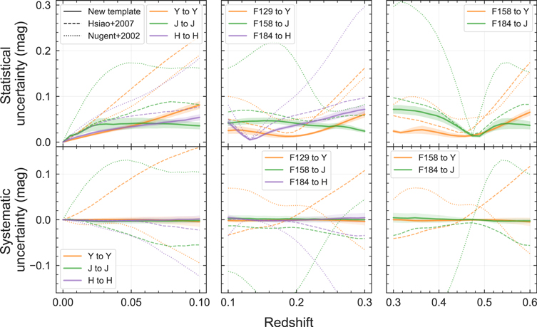
Figure 16. K-correction uncertainties of the new template compared to those of the Nugent (Nugent et al. 2002) and Hsiao (Hsiao et al. 2007) templates. The rms and the mean of the K-correction differences between the template and observed spectra are taken as the statistical (top panels) and the systematic (bottom panels) uncertainties. The mean and standard deviation of the 1000 iterations are shown as solid curves and shaded regions, respectively. (See the text for details.) The filters used are the YJH scans of du Pont + RetroCam, as well as the proposed RST + WFI F129, F158, and F184 filters.
Download figure:
Standard image High-resolution imageAs shown in the upper panels of Figure 16, the statistical K-correction uncertainties of the new template are significantly reduced compared to the previous templates. For example, at z = 0.05, improvements of 0.09, 0.03, and 0.02 mag in the Y, J, and H bands, respectively, can be gained by switching from the Hsiao template to the new one. Note that the result of Boldt et al. (2014) that the smallest uncertainties can be found in the Y band is not reproduced here. From a larger sample, we found that all YJH bands yield similar uncertainties. For cross-filter K-corrections, a minimum would be present at a redshift where the observed and rest-frame filters are aligned (Kim et al. 1996). On average, there is a 0.02 mag improvement in statistical uncertainty compared to the Hsiao template in cross-filter K-corrections.
The lower panels of Figure 16 demonstrate that the systematic K-correction uncertainties are essentially eliminated by adopting the new template. This is true for all of the redshifts and filter combinations considered here, and represents as 0.1 mag improvements in some cases. The improvements in the Y band are the most evident. Since the broadband colors of the template spectra were matched to the observed spectra before the comparison, these uncertainty estimates indicate the ability of the template to predict the spectral feature profile shapes.
4.3. Impact on Cosmology
Here, we explore the impact of adopting the new SN Ia NIR spectral template on cosmological analyses, both at low (e.g., Hubble constant measurements) and high (e.g., dark energy measurements) redshifts.
We first examine the impact on the NIR peak magnitude of adopting the new template on the low-redshift end in single-filter K-corrections. The results are presented in comparison to the Hsiao template in Figure 17. Note that we chose to make the calculations at B-band maximum for convenience, and the analysis yielded a rough estimate of potential magnitude change around peak magnitude. Both templates are scaled and color-corrected to match the YJH magnitudes of the SNooPy light-curve template, which is a function of sBV . Recall that the Hsiao template at peak is a single spectrum and does not account for the variation of spectral features. The spread of roughly 0.1 mag in K-corrections at z = 0.1 results entirely from color corrections.
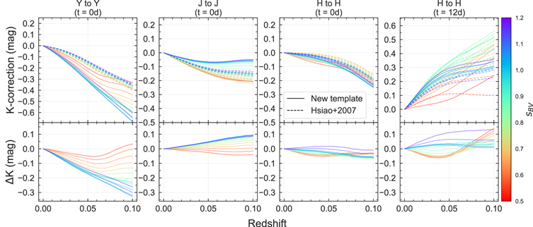
Figure 17. The K-corrections of our new template compared to the previous Hsiao template (Hsiao et al. 2007; Hsiao 2009) at maximum light  . Both templates are color-corrected to match the SNooPy light-curve templates, which is a function of sBV
. The bottom panels plot the K-correction differences between the two templates: ΔK = K(New template) − K(Hsiao). Note that the variation in K-corrections of the new template is caused by both the diversity of the temporal spectral features and the broadband colors, while the variation of the Hsiao template is only reflecting the color variation of the SNooPy light-curve templates in sBV
. The K-correction differences can be substantial, such as for slow decliners at redshift ∼0.1, the ΔK in the Y band is as large as 0.3 mag.
. Both templates are color-corrected to match the SNooPy light-curve templates, which is a function of sBV
. The bottom panels plot the K-correction differences between the two templates: ΔK = K(New template) − K(Hsiao). Note that the variation in K-corrections of the new template is caused by both the diversity of the temporal spectral features and the broadband colors, while the variation of the Hsiao template is only reflecting the color variation of the SNooPy light-curve templates in sBV
. The K-correction differences can be substantial, such as for slow decliners at redshift ∼0.1, the ΔK in the Y band is as large as 0.3 mag.
Download figure:
Standard image High-resolution imageOn the other hand, the new template at peak is a series of spectra that are a function of sBV . Figure 17 shows the difference between the two templates in terms of the K-correction as a function of redshift. It essentially reflects the fact that the diversity is not only in the broadband colors but also in the spectral features. Not accounting for the variation of spectral features as a function of sBV can cause errors in K-corrections as large as 0.3 mag in Y and 0.1 mag in J at z = 0.1. Also note that the two templates show the largest difference in slow decliners (high sBV values). The prominent H-band feature is at maximum strength around 12 days after the maximum. Both slow and fast decliners show K-correction differences as large as 0.1 mag at z = 0.1.
For cosmological analyses using distant SNe Ia, the redshift evolution of the SN Ia population is an important factor to consider. Based on previous high-redshift surveys, the SN Ia population at high redshifts tends to comprise slower decliners and have higher optical light-curve stretch values on average (e.g., Howell et al. 2007; Nicolas et al. 2021). This would introduce an additional systematic shift in the K-corrections if the template SEDs do not reflect the spectral feature variations with light-curve shape.
We simulate such a scenario, considering a shifting sBV distribution at three different redshifts. In the left panels of Figure 18, three populations of SNe Ia are presented at three different redshifts, simulating the distribution of SN Ia light-curve shapes observed locally and at high redshifts (Howell et al. 2007; Riess et al. 2007). The mean of the sBV distributions shifts by as much as 5% from the local sample to z = 1.12. We then calculated K-corrections to the rest-frame Y band and examined the difference between the new and Hsiao templates at B-band maximum.
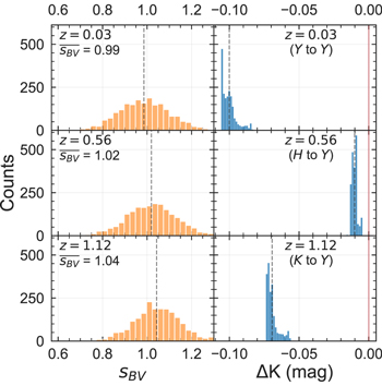
Figure 18. Simulating the effects of an evolving sBV distribution as a function of redshift. Left panels: three redshift bins are considered: one local and two at high redshifts. The sBV distributions are assumed to be Gaussian with the mean converted from the stretch values taken from Howell et al. (2007). The vertical dashed lines mark the mean of the distribution in each bin. Right panels: the distributions of the resulting peak-magnitude K-correction differences are shown, assuming the distribution of sBV in the corresponding left panel. The definition of ΔK is the same as in Figure 17. The vertical dashed lines mark the mean of the distribution in each panel. The red solid vertical line marks the position of ΔK = 0.
Download figure:
Standard image High-resolution imageThe resulting K-correction differences from the corresponding sBV distribution are presented in the right panels of Figure 18. The observer-frame filters for the two high-redshift bins, H and K, align well with the rest-frame Y band at each redshift. The effective wavelength of the de-redshifted H (z = 0.56) and K (z = 1.12) bands match that of the rest-frame Y band within 0.02 μm. Even so, the K-correction differences are systematic and significant, with means of 0.10, 0.01, and 0.07 mag at z = 0.03, 0.56, and 1.12, respectively. The results again highlight the importance of accounting for the spectral feature variations as a function of light-curve shape (e.g., Jones et al. 2022).
5. Conclusion
We present 339 NIR spectra of 98 SNe Ia observed with Baade + FIRE by the CSP-II (Hsiao et al. 2019; Phillips et al. 2019), the largest and the most homogeneous NIR spectral sample of SNe Ia to date. Among those, 331 spectra of 94 SNe Ia were used to construct the most accurate NIR spectral template as a function of a light-curve-shape parameter. The spectra maintain a spectrophotometric accuracy on the level of 10%–20%, allowing for examination of the broadband colors along with the spectral features. The telluric regions are crucial when we study SNe Ia at a range of redshifts. Thankfully, the high-throughput nature of the FIRE NIR spectrograph enables consistent and reliable telluric corrections for ∼70% of the sample.
The aim is to obtain an accurate description of the SN Ia SED in the NIR as a function of phase and sBV . To achieve this, we first utilized PCA to reduce the dimensionality of the data set, then used GPR to model the hypersurface in phase and sBV space. The wavelength grid was divided into seven regions in order to fully utilize the sample and to avoid the PCA results being dominated by spurious pixels or intrinsically high flux. The GPR R2 score has proven to be an efficient metric for selecting which PCs to include for the reconstruction of the SED, capturing the most data variation while using the least number of PCs. The GPR approach also allowed the estimation of the flux uncertainty for each template SED.
The new template successfully captures the diversity of the broadband colors and spectral features as a function of phase and sBV . The hallmark SN Ia NIR features, such as Mg ii at early times and the H-band break past maximum, are recreated in the template SED. In NIR, SNe Ia have more spectral variation than in the optical that cannot be simply described by the varying speed of the evolution for SNe Ia with a range of decline rates. The template is also able to predict the SED shapes of spectra that are not in the training sample and produce photometric colors consistent with the SNooPy light-curve model. Using the cross-validation method, randomly splitting the sample into training and testing sets, a drastic decrease in the K-correction uncertainty is shown compared to previous templates. The new template essentially eliminates any systematic K-correction uncertainties with a 90% improvement compared to the Hsiao template (Hsiao 2009). Simulations of low- and high-redshift cosmological analyses illustrate problems with assuming a fixed template that does not vary with sBV .
The new spectral template will be implemented in SNooPy 38 (Burns et al. 2011) and is available on GitHub 39 along with the source code. It can also be adopted as the baseline SED for other light-curve fitters, such as BayeSN (Mandel et al. 2009, 2011, 2022). As the template fully captures the spectral behaviors of normal SNe Ia, the PCs can be used to identify peculiar features, interesting physics, and possible secondary parameters that could improve their cosmological utility. It will, for example, be revealing to cross-compare these NIR-based PCs with the three-parameter nonlinear parameterization of the optical spectral behaviors of SNe Ia developed by Boone et al. (2021a) from a similarly untargeted sample of 173 SNe, which leads to a much improved (σ ∼0.08 mag) dispersion in cosmological distance measurements (Boone et al. 2021b). The machine-learning techniques developed here will also have a wide range of applications for detecting and modeling the variation in a large and multidimensional data set. Finally, understanding the NIR spectral diversity represents a crucial step forward for future SN Ia cosmological experiments, such as that to be conducted on the Nancy Grace Roman Space Telescope.
The authors would like to thank the referee for providing helpful comments. We thank the technical, scientific staff, and support astronomers of the Las Campanas Observatory for all of the support over the years. The CSP-II has been supported by NSF grants AST-1008343, AST-1613426, AST-1613455, AST-1613472, and the Danish Agency for Science and Technology and Innovation through a Sapere Aude Level 2 grant (PI: M.S.). We thank Prof. Sean Dobbs and Dr. Daniel Lersch for the useful discussion. The Aarhus supernova group is funded by an Experiment grant (No. 28021) from the Villum FONDEN, and by a project 1 grant (No. 8021-00170B) from the Independent Research Fund Denmark (IRFD). C.A. acknowledges STSci grant JWST-GO-02114.032-A. C.G. is supported by a research grant (25501) by the VILLUM FONDEN. E.B. acknowledges NASA grant 80NSSC20K0538 and STSci grant JWST-GO-02114.032-A. L.G. acknowledges financial support from the Spanish Ministerio de Ciencia e Innovación (MCIN), the Agencia Estatal de Investigación (AEI) 10.13039/501100011033, and the European Social Fund (ESF) “Investing in your future” under the 2019 Ramón y Cajal program RYC2019-027683-I and the PID2020-115253GA-I00 HOSTFLOWS project, from Centro Superior de Investigaciones Científicas (CSIC) under the PIE project 20215AT016, and the program Unidad de Excelencia María de Maeztu CEX2020-001058-M. S.G.G. acknowledges support by FCT under project CRISP PTDC/FIS-AST-31546/2017 and project No. UIDB/00099/2020.
Facilities: Magellan Baade Telescope (FIRE) - , Swope Telescope - .
Software: Astropy (Astropy Collaboration et al. 2013, 2018), Pandas (McKinney et al. 2010; Pandas Development Team 2020), PyTorch (Paszke et al. 2019), scikit-learn (Pedregosa et al. 2011), SNooPy (Burns et al. 2011).
Appendix A: NIR Spectra Sample Tables
In this work, we publish 339 NIR spectra of 98 SNe Ia obtained by the CSP-II that passed the first two selection criteria outlined in Section 2.1. Table A1 presents the information of the SNe Ia and spectra. Note that the  and the sBV
of the sample SNe were obtained by fitting multiband CSP light curves with SNooPy. The phases are relative to
and the sBV
of the sample SNe were obtained by fitting multiband CSP light curves with SNooPy. The phases are relative to  . The spectral data and the information in this table are available in the CSP website (https://csp.obs.carnegiescience.edu/data).
Table A1. Summary of SNe Ia and Spectra Used in This Work
| SN Name | zhelio |

| sBV | Spec | UT Date | MJD | Phase | Exp. a | S/N |
|---|---|---|---|---|---|---|---|---|---|
| (MJD) | Counts | (day) | (day) | (s) | (in H) | ||||
| ASASSN-14ad | 0.0264 | 56692.70 ± 0.50 | 1.013 ± 0.040 | 6 | 2014-2-8 | 56696.40 | 3.6 | 571 | 10 |
| 2014-2-15 | 56703.39 | 10.4 | 1141 | 2 | |||||
| 2014-2-22 | 56710.32 | 17.2 | 380 | 8 | |||||
| 2014-2-27 | 56715.31 | 22.0 | 1014 | 13 | |||||
| 2014-3-10 | 56726.23 | 32.7 | 1014 | 16 | |||||
| 2014-3-25 | 56741.25 | 47.3 | 1522 | 8 | |||||
| ASASSN-14hp | 0.0389 | 56929.53 ± 0.06 | 1.077 ± 0.041 | 1 | 2014-11-5 | 56966.13 | 35.2 | 1522 | 6 |
| … | … | … | … | … | … | … | … | … | … |
| iPTF14w | 0.0189 | 56669.93 ± 0.03 | 0.743 ± 0.040 | 7 | 2014-1-9 | 56666.34 | −3.5 | 507 | 42 |
| 2014-1-14 | 56671.31 | 1.4 | 507 | 20 | |||||
| 2014-2-8 | 56696.36 | 25.9 | 1014 | 28 | |||||
| 2014-2-15 | 56703.33 | 32.8 | 1522 | 6 | |||||
| 2014-2-22 | 56710.24 | 39.6 | 1522 | 10 | |||||
| 2014-2-27 | 56715.27 | 44.5 | 1014 | 9 | |||||
| 2014-3-18 c | 56734.13 | 63.0 | 1522 | 24 | |||||
| … | … | … | … | … | … | … | … | … | … |
| SN 2013hn b | 0.0151 | 56642.94 ± 0.69 | 0.821 ± 0.048 | 4 | 2013-12-20 | 56646.36 | 3.4 | 888 | 47 |
| 2013-12-27 | 56653.35 | 10.3 | 761 | 21 | |||||
| 2014-1-1 | 56658.35 | 15.2 | 634 | 52 | |||||
| 2014-1-14 | 56671.34 | 28.0 | 507 | 33 | |||||
| … | … | … | … | … | … | … | … | … | … |
Notes. This table is published in its entirety in machine-readable format. A portion is shown here for guidance regarding its form and content.
a Total on-target exposure time excluding overhead. b SNe discovered by targeted search. c Spectra not included in the final sample for template construction due to host contamination.Only a portion of this table is shown here to demonstrate its form and content. A machine-readable version of the full table is available.
Download table as: DataTypeset image
Appendix B: Alternative Method: Conditional Variational Autoencoder
As we mentioned in Section 3, the current PCA+GPR method has some limitations. Here we propose an alternative machine-learning method, using extensions of the autoencoder network, that could circumvent the drawbacks in the current approach.
Autoencoders have been employed in astronomy with rising popularity in recent years (e.g., Villar et al. 2020; Boone 2021; Gabbard et al. 2022). An autoencoder is a type of neural network architecture that couples an encoder neural network and a decoder neural network, with some reduction in dimensionality at their connection point. This reduced space is known as the latent space of the network, and can be seen as a nonlinear subspace, in comparison with the linearly transformed subspace that is formed from PCA. The dimensionality of the latent space is akin to the choice of the number of PC dimensions used for template generation. The network is forced to reconstruct the inputs utilizing the fewest dimensions while incurring some reconstruction loss that can be minimized.
A variational autoencoder (VAE; Kingma & Welling 2013) extends its predecessor by encoding for random variables. Typically, this is chosen to be a vector of means and variances for a set of Gaussian random variables. Decoding random samples from the latent space gives access to the probability density function of generated templates. An additional regularization (Kullback–Leibler divergence) term is added to the loss function of the standard VAE architecture that attempts to maintain some level of continuity in the latent space by guiding the embeddings to be more Gaussian distributed. This makes template generation smoother. Furthermore, an extension to the VAE architecture can be made by conditioning the encoder and decoder on external variables, e.g., phase and sBV . This addition is known as a conditional VAE (cVAE; Sohn et al. 2015) and allows us to output template spectra for given phase and sBV inputs continuously, without requiring an additional GPR step.
Here, a cVAE for template generation is implemented in the pyTorch (Paszke et al. 2019) framework, and its performance will be analyzed. The encoder is constructed as a feed-forward neural network consisting of four layers containing 3673, 128, 32, and 5 nodes, respectively. Rectified linear units are used as activations. The decoder neural network, in this case, mirrors the encoder with the exception that the first node contains 5 + 2 nodes (the +2 is reserved for conditioning the decoder on the template parameters). The cVAE is optimized using the Adam optimizer (Kingma & Ba 2014) with a learning rate of 10−3 and a batch size of 16. The model is trained for 500 iterations. Under the current settings, the computation time of cVAE is four times longer than the PCA+GPR method, at around 40 minutes and 13 minutes, respectively. However, the time would depend on the hardware and the choice of iterations.
Figure B1 shows a comparison of the templates generated by PCA+GPR and the proposed cVAE method. The current PCA+GPR method still provides the best results, with a median χ2/dof of 1.43 while compared to observed spectra (see Section 3.4). The templates constructed with cVAE method yield a median χ2/dof of 1.76. The current data set might not be large enough to train the cVAE to adequately separate the signal from the noise, especially in the telluric regions and the noisy edge of the K band. Further exploration, such as refining selection criteria and training for more iterations, is required to further investigate the causes of deficiencies in these regions.
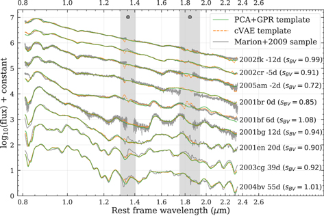
Figure B1. Comparisons between templates constructed using the current PCA+GPR method (green solid lines) and the cVAE method (orange dotted lines). Selected observed spectra from Marion et al. (2009), which are not included in the training process of either template, are also presented in the background for comparison (gray solid lines). All comparison spectra are color-corrected to match the broadband colors. The regions of the strongest telluric absorptions are marked with vertical gray bands.
Download figure:
Standard image High-resolution imageHowever, there are caveats in this comparison of the resulting templates. The input data of cVAE and the PCA+GPR method do not have the same structure: the input data of cVAE is not split into wavelength regions, and the input data is normalized in both mean and standard deviation, whereas the input data for PCA is only normalized by mean in each column. Additionally, only ∼70% of the sample is included for training in the cVAE approach due to the limitation of the reliable telluric regions, which essentially reduces the training size by 30% in the zYJH and 20% in the K band compared to the PCA+GPR method.
The proposed cVAE architecture requires fixed wavelength grid as an input, similar to PCA. A useful extension to this would be to support sequence inputs of varying length, thereby skipping any implicit biases that can be introduced by the interpolation preprocessing step. One clear and natural pathway forward would be to incorporate long short-term memory or recurrent neural network nodes. Here, a single node takes in an entire sequence, element by element, and contains an internal state that allows information from previous elements of a sequence to affect the output for the next element. Using a sequence approach is also beneficial in that different regions can be ignored, e.g., wavelength regions that have poor telluric corrections.
In summary, the cVAE approach has the following potential advantages over PCA+GPR: it can naturally deal with irregular/missing data and unifies the two-step PCA+GPR procedure allowing the template generation and dimensionality reduction steps to communicate. However, it appears that a larger data set is needed to better harvest the potential of this method.
Appendix C: Gaussian Process Regression Kernel Parameters
In this section, we present the details of the GPR kernel setup and the optimal kernel parameters, as well as a demonstration of how the length scales of the RBF kernel affect the template spectra.
In Section 3.3, GPR was used to establish the average dependence of the PC projection values on phase and decline rate,  . With
  , one can “look up” the PC projections and construct the average SED of an SN Ia for any particular value of sBV
and phase. GPR has the advantage of being nonparametric, in the sense that no particular functional form is chosen to represent
, one can “look up” the PC projections and construct the average SED of an SN Ia for any particular value of sBV
and phase. GPR has the advantage of being nonparametric, in the sense that no particular functional form is chosen to represent  . Rather, GPR determines a mean function that is constrained by the data and a covariance function, called the kernel, that controls the amplitude and scale over which this function can vary.
For the kernel, we choose the sum of an RBF covariance function and a white noise term, which has four free hyperparameters and can be represented by the following:

C is a constant, representing the amplitude of the RBF kernel, ℓphase and  are the length scales of the RBF kernel for phase and sBV
, and σ is the noise level of the white noise kernel, W. The best values of these hyperparameters are determined by scikit-learn by maximizing the log-marginal likelihood. All four parameters are given uniform priors.
are the length scales of the RBF kernel for phase and sBV
, and σ is the noise level of the white noise kernel, W. The best values of these hyperparameters are determined by scikit-learn by maximizing the log-marginal likelihood. All four parameters are given uniform priors.
The shape of the probability hypersurface is a complicated one, with obvious degeneracies. The most severe occurs when σ becomes larger than the variations due to sBV
and/or phase. In this case, the RBF scales (ℓphase and/or  ) no longer matter and therefore do not converge to fixed values. In these cases, the resulting
  are simply constant with respect to phase and/or sBV
.
are simply constant with respect to phase and/or sBV
.
The optimal kernel parameters of all GPRs are presented in Figure C1. Around half of the GPRs, especially those of the lower-rank PCs, do not have converged length scales, in which case we set the scale equal to 105, effectively making the GPR independent of that parameter. However, our PC selection strategy (GPR R2 ≥ 0.2; see Section 3.4) was able to screen out the vast majority of GPR fits that have these convergence issues. The only selected PC that has not fully converged is PC1 of the W4 (telluric) region, which has an  . In general, for the templates presented in this work, the median optimal length scales of the selected PCs are 18 days and 0.43 for phase and sBV
, respectively. The optimal length scales for phase are similar to the best-fit length scale for the SNooPy light-curve template (∼30 days), which were also constructed with GPR. PCs that have relatively short optimal length scales may indicate spectral features that evolve faster than the photometry, such as those due to ionization changes.
. In general, for the templates presented in this work, the median optimal length scales of the selected PCs are 18 days and 0.43 for phase and sBV
, respectively. The optimal length scales for phase are similar to the best-fit length scale for the SNooPy light-curve template (∼30 days), which were also constructed with GPR. PCs that have relatively short optimal length scales may indicate spectral features that evolve faster than the photometry, such as those due to ionization changes.
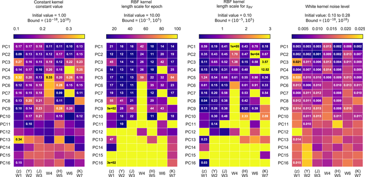
Figure C1. The heatmaps of the optimal kernel parameters of GPRs. From left to right are the constant (C), RBF kernel length scale for phase (ℓphase), RBF kernel length scale for sBV
( ), and white kernel noise level (σ), respectively. The selected PCs for the template constructions with GPR R2 ≥ 0.2 (see Section 3.4) are indicated with labels.
Download figure:
Standard image High-resolution imageWhile our analysis provides optimal values for the four hyperparameters, there are associated uncertainties in their values. It is therefore worth considering the effects of varying each hyperparameter with respect to the constructed SN Ia SED. In other words, how do uncertainties in the hyperparameters propagate to uncertainties in the final SN Ia SED? Since the phase and sBV
are the two input parameters for the template, the temporal spectra are likely to vary with their RBF length scales the most. To illustrate how each of the length scales affects the final template, we keep one length scale at the optimal value, while varying the other by 1σ median absolute deviation (MAD). The MADs of ℓphase and  among selected PCs are 6.6 and 0.22, respectively.
The resulting test templates are shown in Figure C2, where variations in ℓphase are plotted above the data as a sequence from blue to yellow lines, and variations in  are plotted below as a sequence from red to blue lines. On the left, we plot SN 1999by at +14.0 days, which has a decline rate sBV
= 0.42, and on the right, we plot SN 2015 at +47.2 days, which has a decline rate sBV
= 0.67. These were chosen to represent points in the phase-sBV
space that are sparsely sampled by the training data (see Figure 3). SN 1999by, being on the low edge of the sBV
distribution, shows a larger variation when varying
are plotted below as a sequence from red to blue lines. On the left, we plot SN 1999by at +14.0 days, which has a decline rate sBV
= 0.42, and on the right, we plot SN 2015 at +47.2 days, which has a decline rate sBV
= 0.67. These were chosen to represent points in the phase-sBV
space that are sparsely sampled by the training data (see Figure 3). SN 1999by, being on the low edge of the sBV
distribution, shows a larger variation when varying  than in the case of SN2015bp, which resides in a better-sampled part of the sBV
distribution.
than in the case of SN2015bp, which resides in a better-sampled part of the sBV
distribution.
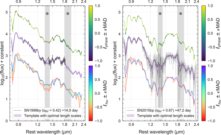
Figure C2. Comparison between the test templates with varying length scales, the observed spectra, and the optimal template. The phase and sBV length scales are varied by 1σ median absolute deviation (MAD) and are plotted on the top and bottom of the observed spectrum, respectively. The template is less robust against varying length scales in regions of the parameter space that are not well modeled, such as sBV = 0.42 (left panel). The right panel shows the same comparison but at sBV = 0.67 and phase = +47.2 days, which is on the border of extrapolation. Note that the spectra are color-matched in this comparison.
Download figure:
Standard image High-resolution imageIt should be emphasized that the “errors” seen in Figure C2 are exaggerated since the real variations in ℓphase and  due to uncertainties are lower (on the order of 0.2 days and 0.1, respectively). Nevertheless, it illustrates that improvements can be made by adding more training data in those areas that are sparsely sampled in sBV
and phase, particularly fast-declining SNe at late phases.
due to uncertainties are lower (on the order of 0.2 days and 0.1, respectively). Nevertheless, it illustrates that improvements can be made by adding more training data in those areas that are sparsely sampled in sBV
and phase, particularly fast-declining SNe at late phases.
Footnotes
- 31
Note that a few FIRE spectra obtained by the CSP-II were taken in the echelle mode.
- 32
- 33
z as Sloan Digital Sky Survey z, YJH as CSP-II du Pont + RetroCam YJH (Phillips et al. 2019), and K as CSP-I du Pont + WIRC KS (Contreras et al. 2010). The CSP filter functions are available on the web at https://csp.obs.carnegiescience.edu/data/filters and in the Python package SNooPy (Burns et al. 2011).
- 34
The initial length scales for the RBF kernel adopted in this work are 10 and 0.1 for phase and sBV , respectively.
- 35
Linear weights were assigned to the flux points such that the spectrum edges have the lowest weights.
- 36
- 37
- 38
- 39