Abstract
Due to the inevitable accumulation of observational information in the direction of the line of sight, it is difficult to measure the local magnetic field of magnetohydrodynamic (MHD) turbulence. However, a correct understanding of the local magnetic field is a prerequisite for reconstructing the Galactic 3D magnetic field. We study how to reveal the local magnetic field direction and the eddy anisotropy on the basis of the statistics of synchrotron polarization derivative with respect to the squared wavelength dP/dλ2. In the low-frequency and strong Faraday rotation regime, we implement numerical simulations in the combination of multiple statistic techniques, such as structure function, quadrupole ratio modulus, spectral correlation function, correlation function anisotropy, and spatial gradient techniques. We find that (1) statistic analysis of dP/dλ2 indeed reveals the anisotropy of underlying MHD turbulence, the degree of which increases with the increase of the radiation frequency; and (2) the synergy of both correlation function anisotropy and gradient calculation of dP/dλ2 enables the measurement of the local magnetic field direction.
1. Introduction
Turbulence is a ubiquitous phenomenon in astrophysical plasmas. Due to the electrical conductivity of plasma astrophysics, turbulent motions of astrophysical fluids are accompanied by magnetic field fluctuations (Biskamp 2003), resulting in the production of magnetohydrodynamic (MHD) turbulence. The most significant observational evidence for turbulence is from the spectral distribution of electron density fluctuations in the Milky Way (Armstrong et al. 1995; Chepurnov & Lazarian 2010). The extra evidence comes from measurements of velocity fluctuations by using Doppler shifted spectral lines (Lazarian 2009, for a review) and magnetic field measurements by synchrotron fluctuations (Cho & Lazarian 2010; Gaensler et al. 2011; Burkhart et al. 2012). Actually, MHD turbulence plays a major role in the key astrophysical processes, such as star formation (mac Low & Klessen 2004; McKee & Ostriker 2007), propagation and acceleration of cosmic rays (Yan & Lazarian 2008), heat conduction (Narayan & Medvedev 2001), and turbulent magnetic reconnection (Lazarian & Vishniac 1999, hereafter LV99). The importance of studying MHD turbulence is that it allows us to understand the processes of astrophysics mentioned above and improve theoretical developments as well.
In recent three decades, traditional theoretical and experimental methods in the study of MHD turbulence have been complemented by numerical simulations providing many valuable results, such as the confirmation of scale-dependent anisotropy (Cho & Vishniac 2000, hereafter CV00) and the compressibility of MHD turbulence (Cho & Lazarian 2002; Kowal & Lazarian 2010). Usually, the Reynolds numbers Re = LV/μ, used for characterizing the level of turbulence, are extremely large in the magnetized astrophysical plasmas, with the large astrophysical scale L and velocity V, but the finite value of kinematic viscosity and magnetic diffusivity μ determined by microphysics. One example is that an order of magnitude Re = 1010 (or larger) is common for the interstellar medium (ISM). However, the present direct numerical simulations are limited to Re ∼ 105, leaving a large gap between the numerical simulation setting and real astrophysical environments. Therefore, it is necessary to develop and use new observation-oriented methods to measure the properties of the ISM, removing the cosmic microwave background (CMB) foreground, exploring the propagation of cosmic rays, and predicting the ratio of star formation.
Many astrophysical phenomena suggest that relativistic electrons are widespread in the cosmos, where interactions of the electrons with the fluctuating magnetic fields lead to synchrotron emission fluctuations carrying important information about magnetization turbulence. By studying synchrotron fluctuations we can obtain basic insights into magnetic fields. We emphasize that how relativistic electrons are accelerated is still an open issue. According to classical shock acceleration theory, a single spectral index of the electrons of 2 was usually assumed in a number of earlier papers. Hence, synchrotron intensity fluctuations are used to extract the spectrum and anisotropies of underlying magnetic turbulence (e.g., Getmantsev 1959; Lazarian & Shutenkov 1990), and polarization fluctuations are used to measure magnetic field helicity (Waelkens et al. 2009; Junklewitz & Enßlin 2011). Adopting an analytical description, Lazarian & Pogosyan (2012, hereafter LP12) derived in detail the correlation of synchrotron fluctuations for an arbitrary spectral index of relativistic electrons and predicted the synchrotron intensity fluctuations anisotropic with significant correlation along the direction of the magnetic field. One of their main findings is that the anisotropy is dominated by the quadrupole moment sensitive to the compressibility of the underlying turbulence, which was confirmed in Herron et al. (2016) using numerical simulations. Recently, the quadrupole ratio modulus has been applied to the study of synchrotron polarization intensity anisotropy (Lee et al. 2019; Wang et al. 2020).
Polarized synchrotron radiation, together with the Faraday rotation measure, known as the Faraday rotation synthesis (Burn 1966; Brentjens & de Bruyn 2005), can provide valuable information on the plane-of-sky geometry of the magnetic field for external galaxies. The difficulty of studying the line-of-sight magnetic field component using this method is obvious (Ferrière 2016) because the sign of the Faraday rotation measure varies due to the direction changes of the line-of-sight magnetic field component. To break the limit of this technique, Lazarian & Pogosyan (2016, hereafter LP16) proposed a series of theoretical predictions of synchrotron polarization fluctuations to reveal the underlying magnetic turbulence, which were confirmed in consequent numerical simulations (Lee et al. 2016; Zhang et al. 2016, 2018) and applied to observations (Xu & Zhang 2016; Guo et al. 2017; see Beresnyak & Lazarian 2019 for a recent book).
The scale-dependent anisotropy of eddies is a significant characteristic of the theory of MHD turbulence (Goldreich & Sridhar 1995, henceforth GS95). The degree of the scale-dependent anisotropy of eddies enlarges as the eddy size gets smaller (GS95), as established by the local magnetic field direction (LV99; CV00), supplemented MHD turbulence theory in later studies (LV99; CV00). We emphasize that maintaining scale-dependent anisotropy is not in the observer (projected mean magnetic field) reference frame, where the largest eddies endow MHD turbulence with scale-independent anisotropy (CV00).
It is in the reference system of the mean magnetic field that theoretical descriptions of both synchrotron intensity (LP12) and polarization intensity fluctuations (LP16) are formulated along the line-of-sight integral. Adopting the eddy description of MHD turbulence (LV99; Cho et al. 2002), the gradients of both velocities and magnetic field are expected to be perpendicular to the local magnetic field direction, motivating the development of gradient techniques of the velocity and synchrotron radiation (González-Casanova & Lazarian 2017; Lazarian et al. 2017). The synchrotron gradient techniques, including synchrotron intensity (Lazarian et al. 2017), polarization intensity, and its derivative with respect to the squared wavelength (Lazarian & Yuen 2018, henceforth LY18), were suggested to trace directions of projected mean magnetic fields. By promoting polarization gradients to various advanced diagnostic quantities derived in Herron et al. (2018a, 2018b), Zhang et al. (2019a, 2019b) found that synchrotron gradient techniques have a significant advantage over the traditional polarization method in tracing projected magnetic fields, and consistent measurements were found for the Galactic magnetic field directions by means of the multifaceted advanced diagnostic gradients.
With 3D data cubes of magnetic fields from numerical simulations, CV00 achieved scale-dependent anisotropy in the local frame of the eddies, using the second-order structure function. However, when it comes to observations, it seems to unable to obtain the local magnetic field due to the inevitable accumulation of observational information in the direction of the line of sight. Reproduction of local magnetic fields is essential to reconstruct Galactic 3D magnetic field structure. As in our previous work, the synchrotron polarization derivative with regard to the squared wavelength dP/dλ2 was predicted analytically by LP16 and confirmed numerically by Zhang et al. (2018) to be sensitive to Faraday rotation. Using statistical analysis of dP/dλ2, this paper studies how to obtain anisotropy of small-scale eddies and trace the direction of the local magnetic field in the event of very low-frequency strong Faraday rotation.
The paper is organized as follows. Section 2 gives brief descriptions on the theory of MHD turbulence, synchrotron radiative processes, and polarization derivative with respect to the squared wavelength, following the description of multiple statistic techniques in Section 3. Section 4 provides a description of the generation and anisotropy analysis of simulation data cubes, with numerical results presented in Section 5. A discussion and a summary are presented in Sections 6 and 7, respectively.
2. Theoretical Fundamentals
2.1. Scale-dependent Anisotropy of MHD Turbulence
Since the hydrodynamic type motions of eddies that mix magnetized fluid give rise to Alfvénic perturbations for the magnetic field, MHD turbulence was usually considered a dynamical process of the turbulent cascade dominated by the Alfvén wave interactions. The Alfvén Mach number, describing the strength of magnetic turbulence, is defined as MA = VL/VA, where VL is turbulent injection velocity at the scale Lin and  is the Alfvén velocity. Correspondingly, the largest turbulent eddies would also reflect the Alfvén Mach number at the injection scale Lin, i.e.,
  with BL being the perturbation of the magnetic field B at the injection scale Lin. Then, the relative perturbations of magnetic fields and eddy velocities are related in a symmetrical way (Lazarian et al. 2020)L

where  is the fluctuation of the magnetic field B at the scale l of the turbulent fluid and vl is the corresponding velocity fluctuation.
The modern theory of MHD turbulence (GS95) can be understood as a collection of anisotropic eddies aligning with the direction of local magnetic fields around them, that is, the motions of the eddies with parallel scales l∥ and perpendicular scales l⊥ are elongated along the direction of the local magnetic field. Assuming that the motion perpendicular to the direction of the local magnetic field has a Kolmogorov scaling of  , the anisotropic relation of eddy scales can be written as

This scaling was originally predicted in the case of strong trans-Alfvénic (MA ∼ 1) incompressible turbulence, with the critical balance condition of  . Later, the GS95 anisotropic scaling (see Equation (2)) was generalized to both MA > 1 and MA < 1 cases (LV99, see also Lazarian 2006). The former is called a super-Alfvénic turbulence regime with VL > VA. In the limiting case of
  , the turbulence presents an essentially hydrodynamic Kolmogorov behavior, i.e., vl = VL(l/Lin)1/3, as the weak magnetic field with lower magnetic energy than kinetic energy has a marginal effect on turbulent dynamics. When vl = VA, the hydrodynamic-like behavior of the turbulence cascade would transition into a strong turbulence regime at the scale
  . In the range from lA to the dissipation scale ldis, the GS95 scaling can be maintained.
The latter, VL < VA, shows weak turbulence ranging from Lin to the transition scale lB = LinMA2, in which the magnetic field fluctuations are quasi-2D and perpendicular to the direction of magnetic fields (LV99, Galtier et al. 2000). At scales less than lB, the relation between the eddy major axis  and its minor axis
  is present again, i.e.,

Setting MA = 1, we recapture the original GS95 relation (see Equation (2)).
In compressible MHD turbulence, the compressible turbulent motions are associated with slow and fast modes (GS95; Lithwick & Goldreich 2001). Numerical simulations (Cho & Lazarian 2002) confirmed that Alfvénic and slow modes have the same anisotropy ( ), while fast modes present an isotropic cascade (
 ).
).
2.2. Synchrotron Polarization Radiative Process
The interactions of relativistic electrons with turbulent magnetic fields emit synchrotron radiation that reveals the properties of magnetic field fluctuations. For simplicity, we consider a homogeneous and isotropic distribution of the electrons with a power-law form of N(γ) ∝ γ2α − 1, where γ is the electron energy and α is a spectral index of the electrons.5 Thus, the synchrotron emission intensity as a function of radiative frequency ν can be written as (Ginzburg & Syrovatskii 1965)
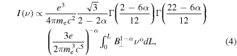
where Γ (x) is a gamma function, B⊥ is the magnetic field component perpendicular to the line of sight, and L is the emitting-region size along the line of sight. Other parameters (e, me, and c) have their usual meanings. With the spectral index of relativistic electrons, we would gain the fraction polarization degree  and the linearly polarized intensity P = pI. The observable Stokes parameters Q and U are related to the polarized intensity by the polarization angle ψ0, i.e.,
  and
and  . When it comes to a Faraday rotation effect, the polarization angle is expressed as
  with the wavelength λ. The Faraday rotation measure
  is given by

Here,  represents a vector in the plane of the sky,
  is the parallel component of the magnetic field, and ne is the thermal electron density.
2.3. Synchrotron Polarization Derivative
With the Stokes parameters Q and U, the complex polarization vector  is formulated as (LP16)

where  indicates the intrinsic polarized intensity density that is treated as wavelength-independent; this simplified treatment would not change the numerical results stated below (see also Zhang et al. 2018 for confirmation).
The condition of decorrelation of the Faraday rotation measure is introduced as

where Leff is an effective spatial depth of the Faraday rotation sampling. Therefore, the ratio of the depth sampled by the Faraday rotation to the emitting-region size can be written as

where  , and σϕ and
  are the root mean square and the mean of the Faraday rotation measure density (
 ) fluctuation, respectively. Using Equation (8), the strong and weak Faraday rotation would be characterized by Leff/L < 1 and Leff/L > 1, respectively. When Leff/L < 1, Equation (6) can be split two parts, in which only z < Leff suffers from the Faraday depolarization, while z > Leff cannot contribute to the polarization measure (see Figure 15 in LY18 for an illustration).
As for a chosen wavelength λ, the complex polarization vector (see Equation (6)) in an effective Faraday depolarization region could be rewritten as

Considering two neighboring wavelengths λ1 and λ2, which respectively correspond to the close spatial positions L1 and L2, we can obtain the differences  and
and  :
:

which reflects the local magnetic turbulence within the ![$z\in [{L}_{2},{L}_{1}]$](https://content.cld.iop.org/journals/0004-637X/895/1/20/revision1/apjab88acieqn26.gif) region. From an observational point of view, providing the Stokes parameters Q and U at two neighboring frequencies, we can obtain the details of the magnetic field fluctuation originating from a locally spatial region. However, note that there is a nonlinear correspondence between L and λ, as expressed in Equation (8). In practice, we consider the statistics of the synchrotron polarization intensity derivative with respect to the squared wavelength,
region. From an observational point of view, providing the Stokes parameters Q and U at two neighboring frequencies, we can obtain the details of the magnetic field fluctuation originating from a locally spatial region. However, note that there is a nonlinear correspondence between L and λ, as expressed in Equation (8). In practice, we consider the statistics of the synchrotron polarization intensity derivative with respect to the squared wavelength,

to reveal the local magnetic field fluctuations.
3. Statistic Measurement Methods
3.1. Correlation and Structure Function Anisotropies
The spatial correlation and structure functions of (any) physical variable  have been traditionally employed for studying anisotropic properties. The former, i.e., the correlation function, is written as

where  denotes an average over the entire volume of interest. As for the latter, the commonly used second-order structure function is given by

It is obvious that the second-order structure function is formally related to the correlation function. Both of them can be used to characterize the eddy anisotropy in MHD turbulence. For the structure function, considering two measurement directions perpendicular to each other, we can define their ratio of individual structure function as

which would reflect the eddy anisotropy of the turbulence structure.
As for the correlation function, it is easy to calculate the correlation function map with a periodic boundary condition through the fast Fourier transform. Studying the non-periodic locality of synchrotron polarization derivative map, we use the Hockney method (Hockney 1968) to solve the open-boundary convolution problem, which helps us decrease computational complexity (Yuen et al. 2018). The direction of the major axis of the correlation (structure) function contour determines the eddy major axis reflecting the magnetic field orientation.
3.2. Spectral Correlation Function
The spectral correlation function (SCF) was initially introduced in Lazarian et al. (2002) to study the anisotropy of turbulence in channel maps of the position–position–velocity 3D space. Here, we adopt this method to explore the correlation of 3D data cubes (as a function of position–position–frequency f(x, y, ν)). The formula used is given by (e.g., Padoan et al. 2003)

where  is a lag vector. The contour of
  would characterize the spatial scales that the spectral features begin to change. The 2D
  correlation can be used to produce the 1D spectrum of the correlation versus the lag length
  by an azimuthal average.
3.3. Quadrupole Ratio Modulus
Following LP12, the normalized correlation function (NCF) of (any) physical variable  can be written as

where  is a separation vector between any two spatial points on the plane of the sky. Similarly, the normalized structure function is expressed as

Therefore, we can obtain the quadrupole moment ratio arising from the variable  ,
,

to reveal the spatial anisotropy, where R is a radial separation and φ is the polar angle.
3.4. Gradient Calculation of 2D Images
In the study of synchrotron gradient measurements, the Sobel operator will be used to compute an approximation of the gradient of the 2D image. This method adopts two 3x3 kernels that are convolved with the original 2D image to obtain approximations of the horizontal and vertical derivatives. And then the recipe of sub-block averaging (Yuen & Lazarian 2017) for the gradient map obtained is used to determine the gradients of the subregion on the 2D image. In each subregion of interest, we use a Gaussian fitting method for the gradient angles to get an optimal direction characterized by the peak of the fitting.
3.5. Alignment Measure
For the magnetic field data cubes obtained by numerical simulation, we can know the intrinsic direction of the underlying magnetic field. Therefore, the magnetic field direction obtained by correlation function anisotropy and gradient techniques can be used to make a comparison with the inherent magnetic field direction. In the case of correlation function anisotropy, the major axis direction of the contour determines the magnetic field direction, whereas in the case of gradient technique, the direction of rotated 90° gradients identifies the directions of the magnetic field.
We adopt a reduction factor to measure the correspondence between the measured magnetic field direction and the intrinsic magnetic field direction (see González-Casanova & Lazarian 2017)

which is called the alignment measure (AM), analogous to the Rayleigh reduction factor in dust alignment theory suggested by Greenberg (1968). The parameter θ in Equation (19) is the angle between the measured magnetic field direction and the intrinsic magnetic fields. AM = ±1 represents a perfect alignment, while AM = 0 no alignment.
4. Magnetic Turbulence Data Generation and Anisotropy Analysis
4.1. Data Generation of Magnetic Turbulence
The following equations are used to describe the interstellar magnetic turbulence environment where the synchrotron radiation is emitted:




Here,  is the gas pressure, t is the evolution time of the turbulent fluid,
  is the current density, and
  is an external driving force. Additionally, an isothermal equation of state would close the above equations.
Numerically, the third-order-accurate hybrid, essentially non-oscillatory code is used to obtain data cubes reaching steady state. In our simulation, an external magnetic field with  is set along the x-axis (horizontal) direction and the random turbulence is driven by a solenoidal driving force at the wavenumber k = 2.5. The resulting 3D data cubes with a numerical resolution of 5123, including the properties of three 3D magnetic fields, three 3D velocities, and one 3D density, are listed in Table 1, where they are depicted by the Alfvénic and sonic Mach numbers.
Table 1. Data Cubes with a Numerical Resolution of 5123 Generated in the Simulation of Compressible MHD Turbulence
| Model | MA | Ms |

|
β |
|---|---|---|---|---|
| run1 | 0.65 | 0.48 | 0.164 | 3.668 |
| run2 | 0.70 | 0.87 | 0.579 | 1.295 |
| run3 | 0.55 | 4.46 | 0.467 | 0.030 |
| run4 | 0.50 | 9.92 | 0.465 | 0.005 |
Note. δ Brms denotes the root mean square of a random magnetic field,  the regular magnetic field, and
  the plasma parameter.
Download table as: ASCIITypeset image
4.2. Anisotropy Analysis of Magnetic Turbulence Data
Adopting a cylindrical coordinate system fixed on the eddies (following CV00), we obtain the local magnetic field via

where  is parallel to the major-axis direction of eddies. In the local reference frame of the magnetic field is the corresponding second-order structure function as

with  and
and  .
.
As a case in point, with the run3 magnetic field data cubes listed in Table 1, Figure 1 shows the structures of scale-dependent anisotropic eddies. The eddy anisotropies in 3D space are plotted in the left panel, while the eddy anisotropies within the 100th 2D slice are plotted along the major and minor axes of eddies (middle panel) and along the x and y axes (right panel), respectively. As seen in Figure 1, the scale-dependent anisotropies of the eddies of MHD turbulence can indeed be revealed in the local reference frame, as predicted in GS95 and confirmed in CV00. The smaller the scale is, the more pronounced the degree of anisotropy is. This figure shows the result of the anisotropic structure of an eddy within a 2D slice, and compares the synchrotron observations presented below. However, even for a plane-like (a slice) geometry, from the synchrotron observational data we have no a priori information about the magnetic field and eddy. As a result, we can study their properties only in the artificially selected “local” coordinate system to observe the eddy structures, as done in the right panel of Figure 1.
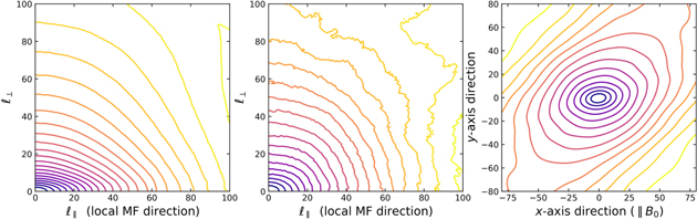
Figure 1. Structures of scale-dependent anisotropic eddies in terms of the run3 magnetic field (MF) data listed in Table 1. The eddy anisotropies in 3D space are plotted in the left panel. The eddy anisotropies within the 100th 2D slice are respectively imaged along the major and minor axes of eddies (middle panel) and along the x and y axes (right panel).
Download figure:
Standard image High-resolution image5. Numerical Results
5.1. Synthesis of Polarized Synchrotron Data Cubes
For the sake of simplicity and for the purposes of simulating real observations and the feasibility of various statistical testing techniques, we consider a scenario with spatially coincident polarized synchrotron emission and Faraday rotation regions, with the assumption of a 1 kpc spatial scale, thermal electron density 0.01 cm−3, and magnetic field strength 1 μG. Focusing on low-frequency observations from the Low Frequency Array for radio astronomy (LOFAR), we can synthesize data cubes of Stokes parameters I, Q, and U ranging from frequencies ν = 10 to 240 MHz in the bandwidth of Δν = 0.46 MHz, on the basis of the 3D simulation data listed in Table 1. This choice of bandwidth can ensure a sufficiently small spatial interval in the line-of-sight direction to achieve successful measurements of the local magnetic field.
Figure 2 depicts the maps at individual frequency points in service of obtaining a qualitative understanding of the synthesized observation data. The upper panels of Figure 2 are the images of synchrotron polarization intensity  , while the middle panels correspond to images of the synchrotron polarization intensity derivative relative to the squared wavelength dP/dλ2. These images are computed for sub-Alfvénic and subsonic turbulence, using the run1 data of Table 1. Their structures are extended along the (x-axis) horizontal direction because the mean magnetic field is set to this direction. We find that the percentage of strong noise-like structure prevents observations at the lowest frequency, 10 MHz. In general, these small-scale structures can be smoothed by a Gaussian filter technique.
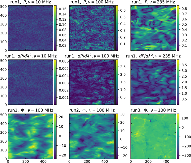
Figure 2. Synchrotron polarization intensities (upper panels) and their derivatives with respect to the squared wavelength (middle panels) in units of mean synchrotron intensity, and Faraday rotation measure (lower panels) in units of rad m−2.
Download figure:
Standard image High-resolution imageThe lower panels of Figure 2 are the images of the Faraday rotation measure, using data cubes from run1 to run3 of Table 1. The values of Faraday rotation measure for sub-Alfvénic and subsonic turbulence (left and middle lower panels) are smaller than those of sub-Alfvénic and supersonic turbulence (lower right panel). In cases of supersonic turbulence, this is caused by the occurrence of high-density (clump) regions arising form shock-wave interactions.
5.2. Spectral Correlation Analysis of the Synchrotron Polarization Derivative
In this section, we adopt the SCF to explore the correlation of multifrequency data cubes as a function of spatial lag separation. Numerical calculation is implemented by extracting the source code from a python package called TURBUSTAT (Koch et al. 2017). With the synchrotron simulation data cubes generated by the run3 listed in Table 1, the resulting image of SCF of dP/dλ2 is shown in the left panel of Figure 3, in which the solid contour line indicates the 2D fitting by an elliptical power-law model, obtaining an optimal index of −0.191. Interestingly, we see the solid contour line extending along the x-axis, which would reflect the mean magnetic field direction. Furthermore, an azimuthal average of the SCF image produces a 1D spectrum of the power-law slope of −0.182 (left upper panel), which is fitted by a linear least-squares method with the weights of the inverse squared standard deviation. We find that the 2D fitting gives a slightly greater index than the 1D fitting.
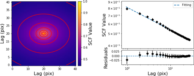
Figure 3. Left panel: image of the SCF value of dP/dλ2 and its fitting (solid line) from an elliptical power-law model, resulting in an index of −0.191. Right panels: an azimuthal average of the correlation surface (left panel) fitted by a linear least-squares method, with a power-law slope of −0.182, from which the inverse squared standard deviation is used as the weights. In the right lower panel are the residuals of the linear fitting. All calculations are based on run3 listed in Table 1.
Download figure:
Standard image High-resolution imageSimilarly, the fitting results of other synchrotron simulation data are as follows: −0.194 (2D) and −0.181 (1D) for run1; −0.175 (2D) and −0.162 (1D) for run2; −0.179 (2D) and −0.172 (2D) for run4. All the above fittings, in the lag range from 1 to 40 pixels, demonstrate the correlation index around −0.2. On the other hand, we also study the possible correlation of SCF values of synchrotron polarization intensity P but find a weak correlation, i.e., a fitting index less than −0.07 for four sets of synchrotron simulation data above. The SCF of P reflects the information of the same projected mean magnetic field measured at different frequencies, while the SCF of dP/dλ2 reveals links between different local magnetic fields. Accordingly, we point out that an SCF analysis of dP/dλ2 can be used to reveal the scale-dependent anisotropies of MHD turbulence. Similar to studies of velocity channel maps (Lazarian et al. 2002), it is expected that the frequency channel maps will reveal more properties of the underlying magnetic field; this will be studied in detail in the future.
5.3. Anisotropy Analysis of the Synchrotron Polarization Derivative
As mentioned in Section 4.2, since an a priori local reference system cannot be fixed on the eddies for observational data, we select the Cartesian coordinate system on the plane of the sky. Figure 4 plots the contour of the structure function of dP/dλ2, which is calculated by run1 of Table 1 at frequencies of 10 MHz ((a) panel), 100 MHz ((b) panel), 200 MHz ((c) panel), and 235 MHz ((d) panel). According to Equation (8), those frequencies are related to the spatial positions 1.4, 134.8, 570.7, and 790.2 pc (a 1 kpc extent length adopted along the line of sight), respectively, where the anisotropic structures of dP/dλ2 qualitatively reflect those of the eddies. Exceptionally, no correlation for the 10 MHz simulation can be seen due to the influence of extremely strong numerical noise.
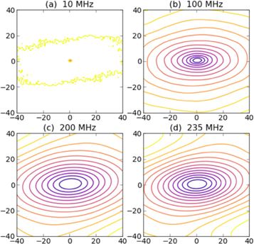
Figure 4. Visualization of the structure function of dP/dλ2, calculated by run1 listed in Table 1 at different frequencies.
Download figure:
Standard image High-resolution imageQuantitative analysis of the structure function of dP/dλ2 is carried out in the left panel of Figure 5, according to Equation (14). As shown, the statistics at high frequencies present stronger anisotropy than those at low frequencies. The degree of anisotropy of dP/dλ2 decreases with increasing spatial scale, which reveals the scale-dependent anisotropy of MHD turbulence (GS95). Moreover, the quadrupole moment ratio (refer to Equation (18)) modulus for dP/dλ2, as a function of the spatial separation, is plotted in the right panel of Figure 5 at the corresponding frequencies. The quadrupole moment ratio moduli decrease with increasing spatial separation, which is generally consistent with the results from the structure function of dP/dλ2 (left panel). In particular, the quadrupole ratio modulus is more sensitive in the anisotropy analysis, as shown in the 10 MHz curves.
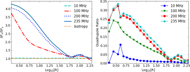
Figure 5. Ratio of the x-axis component to the y-axis component from the structure function of dP/dλ2 (left panel) and the quadrupole ratio moduli of dP/dλ2 (right panel) as a function of the radial separation, calculated by run1 listed in Table 1 at different frequencies. The horizontal dashed line in the left panel represents isotropy.
Download figure:
Standard image High-resolution image5.4. Measurements of Magnetic Field Directions by Correlation Function Anisotropy
On the basis of the analysis of the synchrotron polarization derivative in Section 2.3, the correlation function anisotropy of dP/dλ2 is able to reveal the magnetic turbulence anisotropy of the local spatial region. Measuring the major axis direction of the contour from the correlation function of dP/dλ2, we could trace the local magnetic field direction. Similar to Yuen et al. (2018) and Yang et al. (2020), we rotate the contour map to determine the orientation of the major axis. Compared with the earlier numerical implementation, which was measured at a single spatial point with a rotation step size of 1 degree, this work makes two improvements, including the decrease of the step size to 0.5 degree and the average of the measurement direction of multiple spatial positions.
The alignment measure, between intrinsic directions of the local magnetic fields and directions predicted by the CFA, is shown in Figure 6 as a function of radiation frequency (upper panel) and of the spatial depth along the line of sight (lower panel). In cases of sub-Alfvénic and subsonic turbulence, i.e., MA < 1 and Ms < 1, the CFA can trace the local magnetic field direction apart from the low-frequency part. This is because the presence of strong numerical noise affects the anisotropic distribution of the correlation function of dP/dλ2, and the lack of anisotropy causes CFA not to work. When smoothing the small-scale noise structure in the low-frequency range, we find that AM can be improved to some extent, but this is not shown here. In cases of sub-Alfvénic and super-sonic turbulence, i.e., MA < 1 and Ms > 1, the reverse occurs: numerical noise moves to a lower-frequency part. However, AM values decrease with increasing frequency. In this regard, the formation of a shock wave results in strong density fluctuations. The density-dominated fluctuations should alter the fluctuations of random magnetic fields, leading to the change of the anisotropic structure of the polarization derivative map, on which the CFA tracing is strongly dependent.
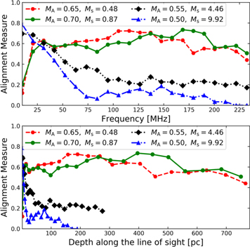
Figure 6. Alignment measure between directions of the local magnetic fields and directions predicted by the CFA as a function of the frequency (upper panel) and of the spatial depth of Faraday rotation sampling (lower panel), on the basis of the data cubes listed in Table 1.
Download figure:
Standard image High-resolution imageAs seen in Equation (8), the relationship between multiple frequencies can be mapped to the local spatial positions in the direction of the line of sight. The lower panel of Figure 6 shows the AM versus the corresponding spatial depth of Faraday rotation sampling. The sampling depth for sub-Alfvénic and subsonic turbulence is greater than that for super-Alfvénic and supersonic turbulence because the high-density fluctuations of the latter (super-) produce stronger Faraday rotation than that of the former (sub-). It is understandable that the strong Faraday rotation sampling depth is shallower. As a result, the CFA is effective for tracing the local magnetic field direction in cases of sub-Alfvénic and subsonic turbulence.
5.5. Measurements of Magnetic Field Directions by Synchrotron Polarization Derivative Gradients
Based on the gradient measurement method stated in Section 3.4, we first compute the gradients of dP/dλ2 by the Sobel operator and divide the whole gradient map obtained into 8 × 8 sub-blocks, each of which has a numerical resolution of 64 × 64 pixels. We then carry out Gaussian fitting for the sub-block gradient map, the peak of which is considered the optimal gradient orientation in each sub-block region. Finally, we average all AMs, and the alignment between the intrinsic magnetic field direction and the gradient one, to obtain an AM value at each frequency.
The resulting AM is plotted in Figure 7 as a function of the frequency (upper panel) and of the spatial depth of Faraday rotation sampling (lower panel), on the basis of four sets of data cubes listed in Table 1. In this figure, most simulations show that AM remains almost unchanged as frequency increases, an exception being the scenario in which the supersonic Mach (Ms ∼ 10) turbulence has an AM that decreases slightly. In particular, the presence of numerical noise approaching 10 MHz does not impede the tracing of the magnetic field direction. It turns out that the synchrotron polarization derivative gradient (SPDG) technique provides the ideal AM for tracing the local magnetic field. In comparison with the results provided in Figure 6 from the CFA measurement (Section 5.4), we find that the capability of the SPDG is greater than that of the CFA in the measurement of magnetic field directions, which is in agreement with studies of velocity gradient techniques (Yuen et al. 2018; Yang et al. 2020). On the other hand, our previous studies demonstrated that the CFA of polarization intensities has the advantage of distinguishing compressible turbulence modes (LP12; Herron et al. 2016; Lee et al. 2019; Wang et al. 2020). Therefore, we believe that the CFA and gradient analysis of the synchrotron polarization derivative are complementary for measurements of magnetic fields.
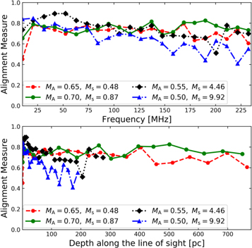
Figure 7. Alignment measure between directions of the local magnetic fields and directions predicted by the SPDG as a function of the frequency (upper panel) and of the spatial depth of Faraday rotation sampling (lower panel), on the basis of the data cubes listed in Table 7.
Download figure:
Standard image High-resolution image6. Discussion
Statistical techniques for finding the synchrotron polarization derivative are motivated by the anisotropic properties of strong MHD turbulence theory (GS95). The empirical evidence strongly supports the GS95 scale-dependent anisotropy  over its competitors. However, we have not addressed discuss what theory can describe the MHD turbulence phenomenon correctly. Our focus is revealing the anisotropic properties of eddies and the direction tracing of the local magnetic field from synchrotron observations rather than confirming the accurate 2/3 scaling relation of GS95. The numerical results presented in this paper are independent of the particular turbulence phenomenology adopted.
In Sections 5.4 and 5.5, no technical improvements were made to the the AM values obtained, such as a smoothing technique, optimizing fitting, or improving sub-block averaging as mentioned in Zhang et al. (2019a), through which the measurement level of the AM would be further enhanced. Using a strong external magnetic field set (B0 > 1, accompanying a strong mean magnetic field  ) to get 3D data cubes in the previous studies of synchrotron gradients (LY18; Zhang et al. 2019a, 2019b), the AM value should be greater to some extent because of its alignment between the projected mean magnetic fields and the 90 degree rotated gradient directions. In this work, the reliability of the measurement results can be ensured when AM is greater than ∼0.6, since all simulations are run with the external magnetic field B0 = 1. Additionally, in the alignment measurement, the gradient technique is more dependent on the resolution of the sub-block than the CFA technique. Further studies are expected to employ higher-resolution data in the future.
We emphasize that magnetic field measurement techniques, such as synchrotron intensity fluctuations (LP12; Herron et al. 2016; Lazarian et al. 2017), synchrotron polarization intensity fluctuations (LP16; Zhang et al. 2016, 2018, 2019a; Lee et al. 2016; LY18), and synchrotron advanced diagnostics statistics (Herron et al. 2018a, 2018b; Zhang et al. 2019b), have been used to investigate the anisotropy caused by the mean magnetic field, the direction of the projected mean magnetic field and the power spectral distributions. Among them, the SPDG technique is proposed to reveal the locally projected mean magnetic field direction within the slices of position–position–position (PPP) data cubes (LY18 and Zhang et al. 2019a). In order to reveal the local magnetic field properties, this work requires a sufficiently narrow frequency bandwidth that corresponds spatially to a single PPP slice, with no projected effect involved. From an observational point of view, our use of a frequency resolution of 0.64 MHz in this paper will not be a problem.
The well-known Faraday tomography method proposed by Burn (1966) defines the Faraday dispersion function as a Fourier transform of the polarization surface brightness with respect to the squared wavelength λ2, aiming at obtaining the properties of intrinsic polarization intensity considered to be a function of Faraday depth (Brentjens & de Bruyn 2005). However, the current statistic measurements related to synchrotron polarization fluctuations define the complex polarized vector as a function of the squared wavelength λ2, and avoid a Fourier transform that would mathematically result in a disorder between the Faraday depth and its transform function. A comparison between Faraday Tomography and synchrotron gradient measurement techniques is made to distinguish the effectiveness of the two techniques (Ho et al. 2019). Our techniques can be seen as a complement to Faraday tomography. It is expected that a synergetic application of these techniques will provide more valuable information about the magnetic field in future studies.
7. Summary
With data cubes generated in numerical simulations, we have investigated the scale-dependent anisotropy of eddies and the local magnetic field direction using the statistics of a synchrotron polarization derivative with respect to the squared wavelength, incorporating the structure function ratio, quadrupole ratio modulus, spectral correlation function, correlation function anisotropy analysis, and gradient measurement. The results are as follows.
- 1.Statistical analysis of dP/dλ2 reveals the scale-dependent anisotropy of underlying MHD turbulence, that is, the smaller the spatial scale is, the more significant the degree of the anisotropy. In addition, the degree of anisotropy revealed increases with increasing radiation frequency.
- 2.SCF analysis of dP/dλ2 can be used to explore the scale-dependent anisotropy of magnetic turbulence. The CFA of dP/dλ2 can trace the underlying local magnetic field direction in cases of sub-Alfvénic and subsonic turbulence.
- 3.Gradient techniques of dP/dλ2 work well in measurements of the local magnetic field direction for sub-Alfvénic, and subsonic and supersonic turbulence regimes.
- 4.Oriented toward the lower-frequency regime, the synergy of dP/dλ2 paves the way for application of LOFAR data cubes to the study of MHD turbulence.
We thank the anonymous referee for the valuable comments that improved our manuscript. J.F.Z. is thankful for the support from the National Natural Science Foundation of China (grants No. 11973035 and 11703020), the Hunan Provincial Natural Science Foundation (grant No. 2018JJ3484), and the Guizhou Provincial Key Laboratory of Radio Astronomy and Data Processing (grant No. KF201803). K.H. acknowledges the support of the National Natural Science Foundation of China (grants No. U1931115, U1731110, and U1731106). J.C. is thankful for support from the National R&D Program through the National Research Foundation of Korea Grants funded by the Korean Government (NRF-2016R1A5A1013277 and NRF- 2016R1D1A1B02015014). A.L. acknowledges the support of NSF grant AST 1715754.
Footnotes
- 5
In our simulations, a power-law energy distribution of the isotropic relativistic electrons is assumed to produce the synchrotron polarization emission. However, the interested reader should note the following possible cases happening in the astrophysical environments. First, a hybrid thermal and non-thermal electron distribution (Mao et al. 2018) occurs due to the turbulence heating and acceleration of electrons, and the resulting temperature is associated with the electron energy distribution that deviates from a Gaussian- or blackbody-like distribution (Mao & Wang 2018). In this regard, we predict that the anisotropy of polarization radiation should be related to the temperature of the electrons accelerated. Second, given that the relativistic electron distribution is anisotropic, such as in the region of strong shocks accompanied by turbulence (called jitter radiation: application to gamma-ray burst (Mao & Wang 2013) and X-ray binary (Zhang et al. 2017)), the anisotropic synchrotron polarization radiation will enhance the polarization degree of synchrotron radiation, leading to more significant anisotropy. This helps us improve the anisotropy analysis of polarization techniques and the ability of magnetic field tracing.