Abstract
The Legacy ExtraGalactic UV Survey (LEGUS) is a multiwavelength Cycle 21 Treasury program on the Hubble Space Telescope. It studied 50 nearby star-forming galaxies in 5 bands from the near-UV to the I-band, combining new Wide Field Camera 3 observations with archival Advanced Camera for Surveys data. LEGUS was designed to investigate how star formation occurs and develops on both small and large scales, and how it relates to the galactic environments. In this paper we present the photometric catalogs for all the apparently single stars identified in the 50 LEGUS galaxies. Photometric catalogs and mosaicked images for all filters are available for download. We present optical and near-UV color–magnitude diagrams for all the galaxies. For each galaxy we derived the distance from the tip of the red giant branch. We then used the NUV color–magnitude diagrams to identify stars more massive than 14 M⊙, and compared their number with the number of massive stars expected from the GALEX FUV luminosity. Our analysis shows that the fraction of massive stars forming in star clusters and stellar associations is about constant with the star formation rate. This lack of a relation suggests that the timescale for evaporation of unbound structures is comparable or longer than 10 Myr. At low star formation rates this translates to an excess of mass in clustered environments as compared to model predictions of cluster evolution, suggesting that a significant fraction of stars form in unbound systems.
1. Introduction
Star formation (SF) plays a major role in shaping the evolution of galaxies. On a small scale, feedback from massive stars affects the surrounding environment via intense stellar winds, ultraviolet radiation fields, chemical processing, and explosions. On a large scale, it governs the macroscopic properties of galaxies. Despite its importance, how galaxies form stars over time, likely in response to both internal and external factors, has not been characterized, nor have we fully understood the link between SF and the global properties of the host galaxies. As a result a universal law that describes SF at all scales is still missing (Dobbs et al. 2011, 2013; Hopkins et al. 2013).
The fragmentation of giant molecular clouds (GMCs) likely causes the formation of stars in a clustered environment (e.g., Larson 1981; Elmegreen & Scalo 2004; Mac Low & Klessen 2004; McKee & Ostriker 2007), and it has been known for a while that a fraction of the newly formed systems is not gravitationally bound (Blaauw 1964; Elmegreen 1983; Clarke et al. 2000; Lada & Lada 2003; Goddard et al. 2010; Portegies Zwart et al. 2010; Gieles & Portegies Zwart 2011). For a long time it was believed that the sudden expulsion of residual gas by feedback was decimating the population of young embedded stellar systems (e.g., infant mortality, Tutukov 1978; Hills 1980; Lada & Lada 2003; Bastian & Goodwin 2006; Parmentier et al. 2008), but the strong correlation between young stellar objects (YSOs) and the hierarchical structure of the interstellar medium (ISM, Testi et al. 2000; Gutermuth et al. 2011; Bressert et al. 2012) suggests that only in a fraction of cases is the star formation efficiency sufficiently high to result in bound stellar systems, with the majority of the stars forming in more dispersed structures throughout the natal GMC (Elmegreen & Elmegreen 2001). This suggests that, at least in some environments, SF may occur on a continuous spectrum of number densities, without the need for a critical density threshold (e.g., Bressert et al. 2010; Parker & Meyer 2012).
The fraction of stars that form in bound star clusters is often quantified as the cluster formation efficiency Γ (e.g., Bastian 2008; Goddard et al. 2010; Adamo et al. 2011; Silva-Villa & Larsen 2011). This parameter provides important information on the process of SF (Elmegreen 2002) and cluster disruption (Gieles et al. 2005) in different environments, and it is also a powerful tracer of the history of star formation in distant galaxies (Miller et al. 1997; Larsen et al. 2001; Goudfrooij et al. 2004; Bastian et al. 2005; Smith et al. 2007; Fedotov et al. 2011).
Observational studies of extragalactic cluster populations highlighted a correlation between Γ and the star formation rate surface density ΣSFR of the host galaxy (Larsen & Richtler 2000; Goddard et al. 2010; Adamo et al. 2011; Silva-Villa & Larsen 2011). This correlation seems to suggest that the short freefall times characteristic of the regions of higher gas density would be sufficient to enable the high star formation efficiencies necessary to form bound systems (Kruijssen 2012).
Several studies have investigated if and how Γ depends on the environment. While investigations of how Γ changes within a galaxy have often carefully characterized the sample of clusters used to derive Γ (e.g., Adamo et al. 2015; Johnson et al. 2016; Adamo et al. 2017; Messa et al. 2018), when comparing results from different galaxies, this has often resulted in combining heterogeneous samples of clusters, whose ages and properties had been derived in non-uniform ways. In this paper we take advantage of the Legacy ExtraGalactic UV Survey (LEGUS, PI Calzetti, GO-13364) to investigate the relation between young massive stars (age < 14 Myr) in the field of the host galaxy and the corresponding population of young star clusters and associations.
LEGUS is a Cycle 21 Treasury program that images 50 nearby (distance ∼3.5–18 Mpc) star-forming galaxies in 5 bands (NUV, U, B, V, I) with the Hubble Space Telescope (HST). LEGUS targets were carefully chosen to span the widest range of morphology, star formation rate (SFR), mass, metallicity, internal structure, and interaction state. For each of the targets ancillary data from the near- (λ = 0.231 μm) and far-UV (λ = 0.153 μm) from GALEX, ground-based Hα + [N ii] data, and data from Spitzer Space Telescope and WISE mosaics (λλ = 3.4–160 μm) are available (a complete description of the LEGUS sample and goals is presented in Calzetti et al. 2015).
The paper is organized as follows. Section 2 describes the observations and the data reduction; the color–magnitude diagrams (CMDs) are presented in Section 3, and the distances of our targets as derived from the tip of the red giant branch (TRGB) are discussed in Section 4. Section 5 discusses Γ as derived from the fraction of massive stars in the field (Γ⋆) as a function of the SFR estimated from the far-UV emission. The summary and conclusions are presented in Section 6.
2. Observations and Data Reduction
2.1. The Data
LEGUS was awarded 154 orbits in Cycle 21 to observe 50 star-forming galaxies with the UVIS channel of the Wide Field Camera 3 (WFC3) in the filters F275W, F336W, and when not already available in the Mikulski Archive for the Space Telescope (MAST) archive, also in the filters F438W, F555W, and F814W. For simplicity, from now on, in the text we will refer to these filters as NUV, U, B, V, and I, respectively. The choice of filters was dictated by the desire to distinguish young massive bright stars from faint star clusters, to derive accurate star formation histories for the stars in the field from CMDs, and to obtain extinction-free ages and masses for the star clusters.
Nearly half of the LEGUS galaxies are sufficiently compact that their far-UV (FUV) effective surface can be mapped with one WFC3/UVIS pointing. For those cases in which the galaxy is slightly larger than the UVIS field of view (FoV), the pointing was optimized to achieve the best coverage possible. Similarly, we tuned the observation position angle to maximize the overlap with archival data (when available). Eleven of the LEGUS galaxies are significantly more extended than the WFC3 FoV. For nine of them we collected multiple pointings along the radial direction to span a wider range of environments.
For each filter we acquired three observations following a three-point dither-pattern with a step of ∼188. We devoted a total integration time of ≥2400 s in the NUV filter and ≥1100 s in U. For 15 targets, where long B, V, and I ACS observations were already available in the MAST archive, the final exposure time in U went up to ≥2400 s. For those galaxies that were not previously observed with ACS in the optical, we used ≥900 s to observe them in B and I, and ≥1100 s to acquire data in V. The observations were designed to reach a depth of mVega(NUV) = 24.5, with a signal-to-noise ratio (S/N) ∼ 6 and comparable depth in the other filters. The log of the observations, complete with data set names, proposal IDs, observing dates and times, coordinates, instruments, filters, and exposure times, is reported in Table 1.
Table 1. Log of the Observations
| Data Set | Proposal ID | Obs. Date | Start Time | R.A. | Decl. | Instrument | Filter | Exp. Time |
|---|---|---|---|---|---|---|---|---|
| (yy mm dd) | (h:m:s) | (2000.0) | (2000.0) | (s) | ||||
| ESO 486-G021 | ||||||||
| icdm06cnq | 13364 | 2013 Sep 06 | 22:14:43 | 05d03m19 |
−25°25′22 |
WFC3 | F275W | 787 |
| icdm06cpq | 13364 | 2013 Sep 06 | 22:30:05 | 05d03m19 |
−25°25′24 |
WFC3 | F275W | 787 |
| icdm06ctq | 13364 | 2013 Sep 06 | 22:45:27 | 05d03m19 |
−25°25′23 |
WFC3 | F275W | 787 |
| icdm06cyq | 13364 | 2013 Sep 06 | 23:53:39 | 05d03m19 |
−25°25′22 |
WFC3 | F336W | 370 |
| icdm06d3q | 13364 | 2013 Sep 07 | 00:02:04 | 05d03m19 |
−25°25′24 |
WFC3 | F336W | 370 |
| icdm06d5q | 13364 | 2013 Sep 07 | 00:10:29 | 05d03m19 |
−25°25′23 |
WFC3 | F336W | 370 |
| icdm06d7q | 13364 | 2013 Sep 07 | 00:19:17 | 05d03m19 |
−25°25′22 |
WFC3 | F438W | 370 |
| icdm06daq | 13364 | 2013 Sep 07 | 00:27:42 | 05d03m19 |
−25°25′23 |
WFC3 | F438W | 370 |
| icdm06dgq | 13364 | 2013 Sep 07 | 01:34:57 | 05d03m19 |
−25°25′24 |
WFC3 | F438W | 216 |
| icdm06djq | 13364 | 2013 Sep 07 | 01:52:19 | 05d03m19 |
−25°25′22 |
WFC3 | F555W | 378 |
| icdm06dlq | 13364 | 2013 Sep 07 | 02:00:45 | 05d03m19 |
−25°25′24 |
WFC3 | F555W | 378 |
| icdm06e7q | 13364 | 2013 Sep 07 | 03:16:15 | 05d03m19 |
−25°25′23 |
WFC3 | F555W | 378 |
| icdm06e9q | 13364 | 2013 Sep 07 | 03:24:58 | 05d03m19 |
−25°25′23 |
WFC3 | F814W | 378 |
| icdm06ebq | 13364 | 2013 Sep 07 | 03:33:24 | 05d03m19 |
−25°25′24 |
WFC3 | F814W | 378 |
| icdm06edq | 13364 | 2013 Sep 07 | 03:41:50 | 05d03m19 |
−25°25′22 |
WFC3 | F814W | 224 |
Only a portion of this table is shown here to demonstrate its form and content. A machine-readable version of the full table is available.
Download table as: DataTypeset image
After five years of operations, charge transfer efficiency (CTE) losses were becoming a concern (Bourque & Kozurina-Platais 2013) for WFC3/UVIS, especially at the shorter wavelengths, where the background is low (Baggett & Anderson 2012). To mitigate the effect of the degrading CTE, we artificially increased the background level of the NUV, U, and B exposures by 12 e− using post-flash. Bias level, superbias, superdark subtraction, post-flash removal, and flat-field correction were applied to each WFC3 image through the standard calibration pipeline CALWF3 version 3.1.2. At the time of the data processing, the pixel-based CTE correction was not included in CALWF3, therefore we used the standalone software routine wfc3uv_ctereverse_parallel.F provided by the WFC3 team (available at the webpage http://www.stsci.edu/hst/wfc3/tools/cte_tools). Pipeline-processed and CTE-corrected ACS/WFC ∗_flc.fits individual images were downloaded directly from the MAST archive.
2.2. Image Alignment
On average the World Coordinate System (WCS) solution in the header of WFC3 data is more accurate than the one found in old ACS data sets. Therefore, we decided to use the information found in the WFC3 B-band images to align and register the individual ∗_flc images with north up and east to the left. When WFC3 B-band data were not available we used the U-band filter as our reference frame.
Each image was aligned using the tweakreg routine. The astrodrizzle routine (Gonzaga et al. 2012) was then used to combine the aligned images for each filter. Each final drizzled image is sky-subtracted and weighted by its exposure time; it is in units of e− s−1 and has a pixel scale of 39.62 mas pixel−1. The routine tweakback was then used to propagate the improved World Coordinate System solution back to the header of the ∗_flc images. Astrodrizzle was also run to identify those pixels that were affected by cosmic rays (CRs) and other spurious signals (such as hot or bad pixels). This information was blotted back to the data quality (DQ) arrays of the affected original frames.
The ACS/WFC data were aligned and drizzled to the UVIS pixel scale. Because of different orientations and pointings, in some cases we had to mosaic multiple ACS images together to maximize the overlap with the WFC3 data. All images are available for download at https://archive.stsci.edu/prepds/legus/dataproducts-public.html. (doi:10.17909/T9J01Z).
2.3. Photometric Reduction
Positions and fluxes for point-like sources were measured via PSF-fitting using the WFC3 and ACS modules of the photometry package DOLPHOT version 2.0, downloaded on 2014 December 12 from the website http://americano.dolphinsim.com/dolphot/ (Dolphin et al. 2002). Each filter was analyzed independently of the others to both maximize the sensitivity to objects of extreme colors, and expedite the data reduction.
The fluxes of all the sources exceeding an initial sigma detection threshold SigFind ≳ 3.0 in the drizzled images were measured on the individual ∗_flc frames. The final photometric analysis was then performed on all the sources with sigma a threshold SigFinal ≳ 3.5.
For the WFC3 data we used the set of PSF libraries whose cores are based on the effective PSF published by the WFC3 team (see the WFC3 website for further information42
), while for the ACS data we used the PSF libraries derived from Tiny Tim (Krist 1995). For each filter the astrometric solution stored in the header of the ∗_flc was used as the starting point for the alignment of the images in a filter, and then we allowed DOLPHOT to use the bright stars in common with the images to further refine the solution. The final alignment among each image was good to ∼001 precision. The same stars were also used to improve the reference PSFs, by minimizing the residuals from the bright stars fitting. The magnitude of each detected star was iteratively improved by taking into account the contribution of the nearby sources.
We ran a series of artificial star tests on a subset of galaxies, characterized by different amounts of crowding and background levels to optimize the DOLPHOT setup. The final set of parameters we used in our analysis is listed in Table 2. Note that because we had applied the pixel-based CTE correction to each individual ∗_flt image, we turned off the DOLPHOT routine that empirically corrects the photometry for the CTE losses.
Table 2. Parameters Used to Run the Stellar Photometry with DOLPHOT
| DOLPHOT PARAMETERS |
|---|
| img?_shift = 0 0 |
| img?_xform = 1 0 0 |
| img?_apsky = 15 25 |
| img?_RAper = 8 |
| img?_RPSF = 10 |
| img?_RSky = 15.0 35.0 |
| img?_RChi = 2.0 |
| RSky0 = 15 |
| RSky1 = 35 |
| RPSF = 10 |
| RCentroid = 2 |
| SigFind = 3.0 |
| SigFindMult = 0.85 |
| SigFinal = 3.5 |
| MaxIT = 25 |
| PSFPhot = 1 |
| FitSky = 3 |
| SkipSky = 2 |
| SkySig = 2.25 |
| NoiseMult = 0.10 |
| FSat = 0.999 |
| PosStep = 0.25 |
| dPosMax = 2.5 |
| RCombine = 1.5 |
| SigPSF = 5.0 |
| UseWCS = 1 |
| Align = 3 |
| WFC3useCTE = 0 |
| AlignIter = 2 |
| Rotate = 1 |
| SecondPass = 1 |
| Force1 = 1 |
| PSFres = 1 |
| psfoff = 0.0 |
| ApCor = 1 |
| WFC3UVISpsfType = 1 |
Download table as: ASCIITypeset image
We recommend users interested in reproducing LEGUS photometry to download both the drizzled-combined ∗_drc and individual CTE-corrected ∗_flc images from the LEGUS webpage https://archive.stsci.edu/prepds/legus/dataproducts-public.html, because DOLPHOT uses the information stored in the DQ arrays of the ∗_flc images to discard bad pixels and cosmic-ray hits. This information is not recorded in the data downloaded from the MAST archive, and this difference can cause up to a 5% difference in the final photometry. In addition, the WFC3 team has recently largely modified the calibration pipeline, to better reflect the difference in quantum efficiency between the two chips of the UVIS channel (Ryan et al. 2016). Our analysis was performed before the changes in the pipeline were introduced.
DOLPHOT went through several changes and updates in the time we processed our data set. These changes did not always correspond to a change in the package version number. To guarantee self-consistent results for users interested in reproducing LEGUS results, or in running tailored artificial star tests, the DOLPHOT version used to reprocess the entire LEGUS data set, as well as the version of PSF libraries, can be downloaded from the LEGUS webpage. The python-based pipeline to automate the photometry is also available for download.
2.4. The Photometric Catalogs
For each star DOLPHOT provides the position relative to the drizzled image, the magnitude, and a series of diagnostics to evaluate the quality of the photometry, including S/N ratio, photometric error, χ2 for the fit of the PSF, roundness (which can be used to identify extended objects), object type (which describes the shape of the source), and an error flag, which is larger than zero whenever there is an issue with the fitting (i.e., because of saturation or extension of the source beyond the detector field of view).
For each galaxy we are releasing several different photometric catalogs that can be downloaded from the MAST archive. In particular we are releasing:
- 1.The five (one for each filter) single-band outputs of DOLPHOT.
- 2.A five-band catalog that includes all the sources with ERRORFLAG = 0, 1, 2 or 3, and magnitudes brighter than 28.5 and has been labeled as v1;
- 3.A five-band catalog that comprises only sources with magnitudes brighter than 30 and with ERRORFLAG = 0. This catalog has been labeled as v2.
In both versions v1 and v2, the five single-band catalogs were cross-matched using the cross-correlation package CataPack.43 Because of the wide range of wavelengths covered by LEGUS, we used the intermediate B filter as the reference frame.
2.5. Selection Criteria
To correctly interpret the properties of the stellar populations found in the LEGUS galaxies, we need to differentiate as much as possible the bona fide apparently single stars from extended objects, blended sources, and spurious detections. To achieve this goal we independently applied to each filter selection criteria based on the photometric error, the shape of the objects, their isolation and the quality of the PSF-fitting, and the roundness.
In both versions of the multiband photometric catalogs we have used a five digit (one digit per filter from NUV to I from left to right) good photometric quality flag (GPQF). In version v1 each digit can range from 0 to 7, and in version v2 it can range from 0 to 5. In both catalogs 0 corresponds to a non-detection. From the sources with magnitudes brighter than 30 we then considered only those whose sharpness deviates less than 1σ from the mean value per magnitude bin. The sources that passed this criterion were flagged with GPQF ge 2, while GPQF = 1 means that either the sharpness deviates more than 1σ from the mean value for that bin of magnitude. Panel (A)) of Figure 1 shows how the sharpness changes as a function of magnitude in the NUV filter for the galaxy NGC 1705. The black points indicate all the sources that are included in version v1 of the photometric catalog, while the two-dimensional histogram shows the sources that passed the selection in sharpness.
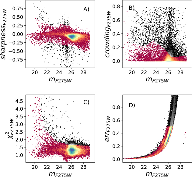
Figure 1. Quality of the photometry for the sources detected by DOLPHOT in the NUV filter for the dwarf galaxy NGC 1705. In each plot all the detected sources are shown as light gray dots, while the two-dimensional histograms highlight the distribution of the sources that passed the selection criteria. Sources were first selected on the basis of their sharpness. Panel (A) is the local crowding, Panel (B) shows sources’ χ2 values, and Panel (C) displays roundness. Panel (D) shows the distribution of the photometric errors.
Download figure:
Standard image High-resolution imageFrom all the sources with “good” sharpness we then selected those whose crowding parameters were less then 2σ from the mean value per magnitude bin, and assigned them GPQFge3. The 2D histogram in Panel (B)) shows the sources that passed both the selection in sharpness and crowding, superimposed on the distribution of all the sources.
Among the sources that passed the selection with crowding, those that are within 3σ from the mean χ2 value in the magnitude bin have been flagged with GPQF ≥ 4 (see Panel (C))), and among these we assigned GPQF = 5 to the sources with photometric error <0.5 (see Panel (C))). A source that passed all the selection criteria in all five bands therefore will have GPQF = 55555, while a source that was detected only in V and I, and that in both filters passed all the selection criteria up to the χ2, will have GPQF = 00044.
In version v1 of the catalog, we applied two further selections: sources with GPQF ≥ 6 are within 1σ from the mean roundness, and sources with S/Ns >2.5 have been flagged with GPQF = 7. For each target the version v1 photometric catalog has the following format: x and y coordinates in the drizzled image reference frame. For each filter we report the magnitude measured in the VEGA system, the photometric error, the reduced χ2 from the PSF-fitting, sharpness, crowding, roundness, S/N, and object type. Filters are listed in order of increasing wavelengths from the NUV to the I band. The ERRORFLAG determined by DOLPHOT have been summarized in column 43 by a 5 digit (one for each filter) ERROR_FLAG. Because 0 corresponds to a non-detection in that filter, we added 1 to the value of the DOLPHOT ERRORFLAG. GPQF is listed in column 44, while right ascension and declination are in columns 45 and 46, respectively. The last column lists a LEGUS-unique identifier. The header of a v1 catalog is shown in Table 3. The version v2 catalogs have the same format, except for the flux, which is not reported.
Table 3. Header of One of the LEGUS Photometric Catalogs
| # | 1 | X_IMAGE | Object position along x | [pixel] |
| # | 2 | Y_IMAGE | Object position along y | [pixel] |
| # | 3 | MAGNI_F275W | WFC3/UVIS/F275W DOLPHOT magnitude in VEGA system | [mag] |
| # | 4 | MAGER_F275W | Magnitude error | [mag] |
| # | 5 | CHISQ_F275W | Reduced chi2 from PSF-fitting | [] |
| # | 6 | SHARP_F275W | Object sharpness | [] |
| # | 7 | CROWD_F275W | Object crowding | [mag] |
| # | 8 | ROUND_F275W | Object roundness | [] |
| # | 9 | SN_F275W | Object S/N | [] |
| # | 10 | OTYPE_F275W | Object type | [] |
| # | 11 | MAGNI_F336W | WFC3/UVIS/F336W DOLPHOT magnitude in VEGA system | [mag] |
| # | 12 | MAGER_F336W | Magnitude error | [mag] |
| # | 13 | CHISQ_F336W | Reduced chi2 from PSF-fitting | [] |
| # | 14 | SHARP_F336W | Object sharpness | [] |
| # | 15 | CROWD_F336W | Object crowding | [mag] |
| # | 16 | ROUND_F336W | Object roundness | [] |
| # | 17 | SN_F336W | Object S/N | [] |
| # | 18 | OTYPE_F336W | Object type | [] |
| # | 19 | MAGNI_F438W | WFC3/UVIS/F438W DOLPHOT magnitude in VEGA system | [mag] |
| # | 20 | MAGER_F438W | Magnitude error | [mag] |
| # | 21 | CHISQ_F438W | Reduced chi2 from PSF-fitting | [] |
| # | 22 | SHARP_F438W | Object sharpness | [] |
| # | 23 | CROWD_F438W | Object crowding | [mag] |
| # | 24 | ROUND_F438W | Object roundness | [] |
| # | 25 | SN_F438W | Object S/N | [] |
| # | 26 | OTYPE_F438W | Object type | [] |
| # | 27 | MAGNI_F555W | WFC3/UVIS/F555W DOLPHOT magnitude in VEGA system | [mag] |
| # | 28 | MAGER_F555W | Magnitude error | [mag] |
| # | 29 | CHISQ_F555W | Reduced chi2 from PSF-fitting | [] |
| # | 30 | SHARP_F555W | Object sharpness | [] |
| # | 31 | CROWD_F555W | Object crowding | [mag] |
| # | 32 | ROUND_F555W | Object roundness | [] |
| # | 33 | SN_F555W | Object S/N | [] |
| # | 34 | OTYPE_F555W | Object type | [] |
| # | 35 | MAGNI_F814W | WFC3/UVIS/F814W DOLPHOT magnitude in VEGA system | [mag] |
| # | 36 | MAGER_F814W | Magnitude error | [mag] |
| # | 37 | CHISQ_F814W | Reduced chi2 from PSF-fitting | [] |
| # | 38 | SHARP_F814W | Object sharpness | [] |
| # | 39 | CROWD_F814W | Object crowding | [mag] |
| # | 40 | ROUND_F814W | Object roundness | [] |
| # | 41 | SN_F814W | Object S/N | [] |
| # | 42 | OTYPE_F814W | Object type | [] |
| # | 43 | ERROR_FLAG | DOLPHOT flags | [0-4] |
| # | 44 | GPQF | Good photometric quality flags | [0-5] |
| # | 45 | ALPHA_J2000 | Right ascension of barycenter (J2000) | [deg] |
| # | 46 | DELTA_J2000 | Declination of barycenter (J2000) | [deg] |
| # | 47 | LEGUS_ID | LEGUS-unique identifier | [LEGUS+HH:MM:SS.SS-DD:MM:SS.S] |
Download table as: ASCIITypeset image
3. Color–Magnitude Diagrams
CMDs are very effective tools for investigating the stellar content of a system, and therefore inferring its star formation history and evolution. Figure 2 shows the optical (I versus V–I, to the left) and NUV (NUV versus NUV-U, to the right) CMDs of the galaxy NGC 4605, obtained from the catalog hlsp_legus_hst_uvis_ngc4605_multiband_v2_stellar_phot.cat. The left panels show only stars with GPQF = ∗∗∗55, while the right panels show only the sources with GPQF = 55∗∗∗.
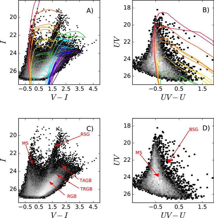
Figure 2. Panel A: optical I vs. V–I CMD for the galaxy NGC 4395. PARSEC isochrones for 4, 8, 16, 40, 100, 250, 630 Myr and 1.6, 4, and 10 Gyr are superimposed in red, dark orange, orange, yellow, green, cyan, light blue, dark blue, purple, and indigo, respectively, by assuming a distance modulus of 28.36, and an extinction E(B–V) = 0.04. Panel B: NUV vs. NUV-U CMD for NGC 4395. PARSEC isochrones for 4, 8, 16, 40, 100 Myr are shown in red, dark orange, orange, yellow, and green. Panel C: optical I vs. V–I CMD with the names and position of the main evolutionary sequences highlighted by red dashed lines. Panel D: NUV vs. NUV-U CMD. Only the upper part of the MS and BSG stars are visible. Their locations are roughly indicated by red arrows.
Download figure:
Standard image High-resolution imagePARSEC isochrones (Bressan et al. 2012; Tang et al. 2014; Chen et al. 2015; Marigo et al. 2017) of different ages are superimposed on the CMDs in the two upper panels. In the two lower panels the evolutionary features characteristic of the two CMDs are highlighted for guiding the interpretation.
In the optical, CMD stars brighter than I < 23.5 are distributed along two sequences. The bluer sequence (V − I < 0.5, sometimes called “blue plume”) hosts intermediate- and high-mass young (down to few Myr) main-sequence (MS) stars, and core helium-burning stars at the blue edge of the blue loop (blue supergiants, BSGs). The bright red stars (V − I > 1.5, red plume) are evolved helium-burning red supergiants (RSGs). Intermediate-mass asymptotic giant branch (AGB) stars of a few hundred million years can be seen in all the LEGUS optical CMDs below the red plume. In most of the CMDs it is also possible to note a sharp discontinuity in the luminosity function of the red stars. This corresponds to the tip of the old (age ≳ 1 Gyr) red giant branch (TRGB).
The morphology and difference in color between the red and the blue plumes, as well as the shape of RGB and tip of the asymptotic giant branch (TPAGB), can be used to constrain the metallicity of a galaxy. By comparing the optical CMDs to PARSEC isochrones, we were able to divide the galaxies in the LEGUS sample into six groups: very metal-poor galaxies with metallicity Z ≃ 0.0008, galaxies with metallicity to close the Small Magellanic Cloud (Z ≃ 0.004), galaxies close to the metallicity of the Large Magellanic Cloud (LMC, Z ≃ 0.008), systems whose metallicity is clearly higher than that in the LMC, but not yet solar (Z ≃ 0.01), galaxies with solar metallicity (Z ≃ 0.02), and finally super-solar systems (Z ≳ 0.03). In 78% of the cases our estimates of the metallicity are in good agreement with literature values (see Table 1 in Calzetti et al. 2015). In 5 cases (namely NGC 1313, NGC 1705, NGC 3344, NGC 4248, and NGC 6744) our estimates are significantly higher than what would be derived from the oxygen abundance reported in the literature, while in three cases (NGC 2500, NGC 4605, and NGC 5238) the morphology of the TRGB and the separation between the blue and the red plumes appear to be too tight compared to the oxygen abundances reported in the literature.
The NUV CMD contains high-mass MS stars and evolved blue supergiants (BSG) at the blue edge of the blue loop. The NUV and U filters are very effective at highlighting the sites of the most recent star formation across the various galaxies. On the other hand, at these wavelengths, even for the nearest galaxies, the LEGUS detection threshold limits the lookback time to ≤100 Myr.
NUV and optical CMDs for all the LEGUS galaxies are shown in the Appendix in Figures 5–15. All the CMDs are obtained from version v2 of the photometric catalogs. The NUV CMDs show only stars with GPQF = 55∗∗∗; in the optical CMD only stars with GPQF = ∗∗∗55 are shown. A careful inspection of the optical CMDs for three of the larger spiral galaxies shows that metallicity is increasing moving from the outskirts toward the center. The most prominent example is NGC 5457 (a.k.a M101), in which we find that the colors of the stellar populations in the most external field (NGC 5457nw3) are better reproduced by isochrones for Z = 0.0008; isochrones with metallicity Z = 0.008 are more indicative for the central pointing (NGC 5457c), while for the three intermediate pointings (NGC 5457se, NGC 5457nw1, and NGC 5457nw2) we used isochrones with metallicity Z = 0.004. Similarly, for NGC 628 we used Z = 0.02 for the central pointing (NGC 628c), while Z = 0.008 seams to be more appropriate for eastern pointing (NGC 628e). Similar metallicity gradients have been previously observed in several other spiral galaxies (Munõz-Mateos et al. 2007; MacArthur et al. 2009; Gogarten et al. 2010), and have been interpreted as an indication that large disks have been forming “inside-out.” In this scenario, star formation started in the center, therefore we should find a higher fraction of older stars in the cores of galaxies compared to the outskirts. This would favor a higher metal enrichment of the interstellar medium in the center of the galaxy, and therefore cause the more recently formed stars toward the center to have higher metal abundances than stars formed in the outskirts of the disk.
The galaxies in our sample are affected by different amounts of dust extinction. For each galaxy we used the foreground extinction derived by Schlafly & Finkenbeiner (2011) and the Fitzpatrick (1999) reddening law RV = 3.1. A comparison of the (NUV-U) and (V–I) colors with PARSEC isochrones shows that in most of the cases the upper MS is affected by a higher amount of extinction than just the Galactic foreground extinction. This is consistent with the fact that stars tend to form in dust-rich environments.
The properties of the galaxies studied in the LEGUS project are summarized in Table 4, including the foreground E(B–V), listed in column 7, and the E(B–V) values derived from the comparison of the upper MS colors with the models are reported in column 8. In addition, the table reports the name of the galaxy in column 1, the RC3 morphological T-type is listed in column 2; and stellar and H i masses (expressed in M⊙) are reported in colums 3 and 4, respectively. Column 5 reports the SFR corrected for dust attenuation derived from the Galex FUV flux, assuming a Kroupa initial mass function, and column 6 reports the FUV half-light radius R1/2. The metallicity Z as inferred from the comparison of the optical CMDs with PARSEC isochrones is reported in column 9. Distance moduli and distances with their respective uncertainties are reported in columns 10 to 13 (see discussion in Section 4). Column 14 reports the number of stars more massive that 14 M⊙ found in the field of each galaxy (see the discussion in Section 5).
Table 4. Properties of the LEGUS Galaxies
| Name | T-type | M⋆ | M(H i) | SFR(UV) | FUV R1/2 | E(B–V)0 | E(B–V) | Z | (m–M)0 | Err (m–M)0 | Dist | Err Dist |

|
|---|---|---|---|---|---|---|---|---|---|---|---|---|---|
| (M⊙) | (M⊙) | (M⊙ year−1) | (arcsec) | Mpc | Mpc | ||||||||
| ESO4486 | 2.0 | 7.2e8 | 2.8e8 | 0.0306 | 20.3 | 0.03 | 0.04 | 0.004 | 29.79 | 0.33 | 9.09 | 0.7 | 198 |
| IC 4247 | 2.2 | 1.2e8 | 1.0e1 | 0.005 | 10.0 | 0.06 | 0.06 | 0.0008 | 28.54 | 0.32 | 5.11 | 0.4 | 146 |
| IC 559 o | 4.0 | 1.4e8 | 3.7e7 | 0.0061 | 11.0 | 0.02 | 0.04 | 0.004 | 30.00 | 0.37 | 10.0 | 0.9 | 68 |
| NGC 1291n | 0.1 | 1.5e11 | 2.3e9 | 0.2344 | 0.0 | 0.01 | 0.16 | 0.02 | 28.98 | 0.34 | 6.3 | 0.5 | 120 |
| NGC 1313e | 7.0 | 2.6e9 | 2.1e9 | 0.1607 | 91.4 | 0.08 | 0.12 | 0.008 | 28.11 | 0.32 | 4.2 | 0.34 | 794 |
| NGC 1313w | 7.0 | 2.6e9 | 2.1e9 | 0.2055 | 91.4 | 0.08 | 0.12 | 0.008 | 28.22 | 0.32 | 4.4 | 0.35 | 763 |
| NGC 1433* | 1.5 | 1.7e10 | 5.0e8 | 0.1856 | 74.0 | 0.01 | 0.03 | 0.02 | 29.78 | 0.49 | 9.1 | 1.0 | 187 |
| NGC 1512c* | 1.1 | 1.7e10 | 8.5e9 | 0.6327 | 0.0 | 0.01 | 0.02 | 0.02 | 30.33 | 0.40 | 11.7 | 1.1 | 468 |
| NGC 1512sw1* | 1.1 | 1.7e10 | 8.5e9 | 0.6463 | 0.0 | 0.01 | 0.03 | 0.02 | 30.38 | 0.45 | 11.9 | 1.3 | 130 |
| NGC 1512sw2 o | 1.6 | 4.8e8 | 6.5e7 | 0.0731 | 4.8 | 0.01 | 0.04 | 0.008 | 30.28 | 0.33 | 11.4 | 0.9 | 231 |
| NGC 1566** | 4.0 | 2.7e10 | 5.7e9 | 2.026 | 91.4 | 0.01 | 0.25 | 0.02 | 31.27 | 0.49 | 18.0 | 2.0 | 7323 |
| NGC 1705 | 11.0 | 1.3e8 | 9.4e7 | 0.0706 | 4.5 | 0.01 | 0.03 | 0.008 | 28.59 | 0.32 | 5.22 | 0.38 | 195 |
| NGC 2500 o | 7.0 | 1.9e9 | 8.2e8 | 0.3161 | 49.0 | 0.03 | 0.3 | 0.004 | 30.18 | 0.46 | 10.9 | 1.2 | 2200 |
| NGC 3274 | 6.6 | 1.1e8 | 5.5e8 | 0.0667 | 31.5 | 0.02 | 0.07 | 0.004 | 30.01 | 0.39 | 10.0 | 0.9 | 867 |
| NGC 3344 | 4.0 | 5.0e9 | 2.3e9 | 0.2585 | 91.4 | 0.03 | 0.26 | 0.02 | 29.59 | 0.37 | 8.3 | 0.7 | 3188 |
| NGC 3351* | 3.1 | 2.1e10 | 1.3e9 | 0.9114 | 0.0 | 0.03 | 0.2 | 0.02 | 29.84 | 0.40 | 9.3 | 0.9 | 1475 |
| NGC 3368 o | 1.9 | 4.8e10 | 2.7e9 | 0.644 | 147.0 | 0.02 | 0.2 | 0.02 | 29.96 | 0.56 | 9.8 | 1.3 | 803 |
| NGC 3627* | 3.1 | 3.1e10 | 1.5e9 | 3.242 | 0.0 | 0.03 | 0.27 | 0.02 | 30.14 | 0.54 | 10.7 | 1.4 | 3443 |
| NGC 3738 | 9.8 | 2.4e8 | 1.5e8 | 0.0374 | 16.5 | 0.01 | 0.08 | 0.004 | 28.53 | 0.32 | 5.09 | 0.40 | 197 |
| NGC 4242 | 7.9 | 1.1e9 | 3.5e8 | 0.0642 | 75.0 | 0.04 | 0.05 | 0.02 | 28.61 | 0.24 | 5.3 | 0.3 | 41 |
| NGC 4248 | 3.3 | 9.8e8 | 6.1e7 | 0.0114 | 29.0 | 0.02 | 0.25 | 0.02 | 29.17 | 0.32 | 6.82 | 0.51 | 98 |
| NGC 4258n | 4.0 | 2.9e10 | 7.3e9 | 1.357 | 0.0 | 0.02 | 0.2 | 0.008 | 29.17 | 0.34 | 6.83 | 0.54 | 2192 |
| NGC 4258s | 4.0 | 2.9e10 | 7.3e9 | 1.357 | 0.0 | 0.02 | 0.2 | 0.008 | 29.17 | 0.34 | 6.83 | 0.54 | 2896 |
| NGC 4395n | 8.9 | 6.0e8 | 1.8e9 | 0.2256 | 0.0 | 0.02 | 0.03 | 0.004 | 28.32 | 0.32 | 4.62 | 0.2 | 149 |
| NGC 4395s | 8.9 | 6.0e8 | 1.8e9 | 0.2154 | 0.0 | 0.02 | 0.04 | 0.004 | 28.22 | 0.32 | 4.41 | 0.33 | 402 |
| NGC 4449 | 9.8 | 1.1e9 | 2.1e9 | 0.5502 | 49.5 | 0.02 | 0.14 | 0.004 | 28.02 | 0.32 | 4.01 | 0.30 | 2206 |
| NGC 4485 | 9.5 | 3.7e8 | 4.0e8 | 0.1846 | 22.5 | 0.02 | 0.11 | 0.004 | 29.71 | 0.35 | 8.8 | 0.7 | 809 |
| NGC 4490 | 7.0 | 1.9e9 | 2.7e9 | 1.119 | 55.0 | 0.02 | 0.25 | 0.004 | 29.06 | 0.35 | 6.5 | 0.5 | 10148 |
| NGC 45 | 7.8 | 3.3e9 | 2.5e9 | 0.2263 | 154.5 | 0.02 | 0.04 | 0.004 | 29.16 | 0.36 | 6.8 | 0.5 | 201 |
| NGC 4594 o | 1.1 | 1.5e11 | 2.8e8 | 0.5502 | 0.0 | 0.01 | 0.22 | 0.02 | 29.99 | 0.47 | 9.9 | 1.1 | 36 |
| NGC 4605 | 5.1 | 1.5e9 | 3.7e8 | 0.2634 | 39.0 | 0.01 | 0.28 | 0.004 | 28.72 | 0.34 | 5.56 | 0.44 | 3059 |
| NGC 4656 | 9.9 | 4.0e8 | 2.2e9 | 0.443 | 173.0 | 0.01 | 0.07 | 0.004 | 29.48 | 0.37 | 7.9 | 0.7 | 1251 |
| NGC 5194c* | 4.0 | 2.4e10 | 2.3e9 | 0.5204 | 91.4 | 0.03 | 0.26 | 0.02 | 29.39 | 0.47 | 7.6 | 0.8 | 2590 |
| NGC 5194ne | 4.0 | 2.4e10 | 2.3e9 | 0.5907 | 91.4 | 0.03 | 0.29 | 0.02 | 29.29 | 0.33 | 7.2 | 0.6 | 3192 |
| NGC 5194sw | 4.0 | 2.4e10 | 2.3e9 | 0.4222 | 91.4 | 0.03 | 0.23 | 0.02 | 29.39 | 0.35 | 7.6 | 0.6 | 1961 |
| NGC 5195* | 2.2 | 2.3e10 | 1.7e9 | 0.2209 | 51.0 | 0.03 | 0.39 | 0.02 | 29.44 | 0.35 | 7.7 | 0.6 | 576 |
| NGC 5238 | 8.0 | 1.4e8 | 2.9e7 | 0.062 | 15.0 | 0.01 | 0.03 | 0.0008 | 28.23 | 0.32 | 4.43 | 0.34 | 54 |
| NGC 5253 | 11.0 | 2.2e8 | 1.0e8 | 0.2635 | 12.0 | 0.05 | 0.16 | 0.0008 | 27.60 | 0.32 | 3.32 | 0.25 | 1103 |
| NGC 5457c | 6.0 | 1.9e10 | 1.9e10 | 3.843 | 0.0 | 0.01 | 0.26 | 0.008 | 28.94 | 0.34 | 6.13 | 0.49 | 2246 |
| NGC 5457nw1 | 6.0 | 1.9e10 | 1.9e10 | 4.513 | 0.0 | 0.01 | 0.16 | 0.008 | 29.29 | 0.33 | 7.2 | 0.5 | 562 |
| NGC 5457nw2 | 6.0 | 1.9e10 | 1.9e10 | 4.213 | 0.0 | 0.01 | 0.16 | 0.004 | 29.14 | 0.32 | 6.7 | 0.5 | 257 |
| NGC 5457nw3 | 6.0 | 1.9e10 | 1.9e10 | 4.213 | 0.0 | 0.01 | 0.16 | 0.0008 | 29.14 | 0.32 | 6.7 | 0.5 | 378 |
| NGC 5457se | 6.0 | 1.9e10 | 1.9e10 | 4.112 | 0.0 | 0.01 | 0.29 | 0.008 | 29.09 | 0.34 | 6.6 | 0.5 | 1636 |
| NGC 5474 | 6.8 | 8.1e8 | 1.3e9 | 0.1638 | 85.5 | 0.01 | 0.23 | 0.004 | 29.08 | 0.32 | 6.6 | 0.5 | 1460 |
| NGC 5477 | 8.8 | 4.0e7 | 1.3e8 | 0.0209 | 27.0 | 0.01 | 0.04 | 0.0008 | 29.13 | 0.32 | 6.7 | 0.5 | 278 |
| NGC 5949 | 4.1 | 1.8e9 | 2.8e8 | 0.1475 | 22.5 | 0.02 | 0.26 | 0.02 | 29.81 | 0.34 | 9.2 | 0.7 | 955 |
| NGC 628c* | 5.2 | 9.2e9 | 9.2e9 | 0.3577 | 91.4 | 0.06 | 0.34 | 0.02 | 29.68 | 0.41 | 8.6 | 0.9 | 3833 |
| NGC 628e | 5.2 | 9.2e9 | 9.2e9 | 0.1483 | 91.4 | 0.06 | 0.24 | 0.008 | 29.73 | 0.34 | 8.8 | 0.7 | 1816 |
| NGC 6503 | 5.8 | 1.9e9 | 1.3e9 | 0.1177 | 91.4 | 0.03 | 0.26 | 0.02 | 28.99 | 0.33 | 6.3 | 0.5 | 1528 |
| NGC 6744c | 4.0 | 2.2e10 | 1.2e10 | 3.999 | 0.0 | 0.04 | 0.13 | 0.02 | 29.23 | 0.40 | 7.0 | 0.53 | 102 |
| NGC 6744n | 4.0 | 2.2e10 | 1.2e10 | 5.031 | 0.0 | 0.04 | 0.19 | 0.02 | 29.73 | 0.39 | 8.8 | 0.8 | 1092 |
| NGC 7793e | 7.4 | 3.2e9 | 7.8e8 | 0.0998 | 91.4 | 0.02 | 0.16 | 0.008 | 27.87 | 0.33 | 3.75 | 0.28 | 1208 |
| NGC 7793w | 7.4 | 3.2e9 | 7.8e8 | 0.0714 | 91.4 | 0.02 | 0.14 | 0.008 | 27.92 | 0.33 | 3.83 | 0.29 | 967 |
| UGC 1249 | 8.9 | 5.5e8 | 9.9e8 | 0.0866 | 97.5 | 0.07 | 0.19 | 0.004 | 29.02 | 0.32 | 6.4 | 0.5 | 931 |
| UGC 4305 | 9.9 | 2.3e8 | 7.3e8 | 0.0816 | 118.0 | 0.03 | 0.06 | 0.008 | 27.55 | 0.32 | 3.32 | 0.25 | 58 |
| UGC 4459 | 9.9 | 6.8e6 | 6.8e7 | 0.0048 | 24.0 | 0.03 | 0.08 | 0.0008 | 27.99 | 0.32 | 3.96 | 0.30 | 38 |
| UGC 5139 | 9.9 | 2.5e7 | 2.1e8 | 0.0125 | 90.0 | 0.04 | 0.07 | 0.0008 | 27.92 | 0.32 | 3.83 | 0.29 | 40 |
| UGC 5340 | 9.7 | 1.0e7 | 2.4e8 | 0.028 | 45.0 | 0.02 | 0.06 | 0.0008 | 30.52 | 0.32 | 12.7 | 1.0 | 751 |
| UGC 685 | 9.2 | 9.5e7 | 9.7e7 | 0.004 | 16.6 | 0.05 | 0.19 | 0.0008 | 28.20 | 0.32 | 4.37 | 0.34 | 36 |
| UGC 695 | 6.0 | 1.8e8 | 1.1e8 | 0.0093 | 7.2 | 0.03 | 0.2 | 0.0008 | 29.45 | 0.32 | 7.8 | 0.6 | 75 |
| UGC 7242 | 6.4 | 7.8e7 | 5.0e7 | 0.0046 | 23.0 | 0.02 | 0.03 | 0.004 | 28.77 | 0.33 | 5.67 | 0.43 | 27 |
| UGC 7408 | 9.3 | 4.7e7 | 8.6e7 | 0.0066 | 25.0 | 0.01 | 0.04 | 0.0008 | 29.23 | 0.33 | 7.0 | 0.5 | 7 |
| UGCA 281 | 10.0 | 1.9e7 | 8.3e7 | 0.0055 | 9.8 | 0.01 | 0.14 | 0.0008 | 28.58 | 0.32 | 5.19 | 0.39 | 119 |
Note. Galaxies for which the derived distance is uncertain have been marked with an asterisk or â symbol. The galaxies used to evaluate the relation between Γ⋆ and the ΣSFR are highlighted in boldface.
The optical CMDs have been corrected for distance, as derived from the luminosity of the TRGB (see Section 4), and foreground extinction. Since the majority of the stars in the NUV CMDs are in the MS evolutionary phase, the NUV CMDs have been corrected for the extra amount of extinction derived from the MS colors. The blue-dotted line in the NUV CMDs marks the luminosity of a M = 14 M⊙ star in the NUV filter for the assumed metallicity, while the dashed line in the optical CMDs highlights the position of the TRGB, as derived in the following section. The galaxies are shown in order of increasing metallicity and SFR.
4. The Tip of the RGB and Galaxy Distance Moduli
The explosive onset of helium-burning in the degenerate core of low-mass stars drastically ends the RGB evolutionary phase. At low metallicity this occurs at about the same brightness for all low-mass stars, and in the I versus V–I CMD this causes a sharp cutoff in the star counts, the so-called TRGB. The luminosity of the TRGB is a standard candle and it has been used to determine the distances of galaxies for more than 35 years (Iben & Renzini 1983; Da Costa & Armadroff 1990; Lee et al. 1993; Sakai et al. 1996). Distances derived from the luminosity of the TRGB agree with those inferred from the Cepheid period–luminosity relation at the level of 0.01 mag (Rizzi et al. 2007).
Several studies have demonstrated that in order to obtain a robust determination of the TRGB, it should be at least one magnitude above the detection threshold (e.g., Madore & Freedman 1995; Makarov et al. 2006; Madore et al. 2009). So far the TRGB has been used to determine the distance of galaxies closer than 18–20 Mpc (Aloisi et al. 2007; Tully et al. 2016)
For low metallicities ([Fe/H] < −0.7), the luminosity of the TRGB in the I band is independent of the age of the stellar population, and the effect of metallicity is less than 0.2 mag (Lee et al. 1993; Salaris & Cassisi 1997; Bellazzini et al. 2001). At higher metallicity, the luminosity of the TRGB depends on the age of the stellar population. Rizzi et al. (2007) have shown that this degeneracy can be broken using the color of the RGB. In our analysis we decided to adopt a more conservative approach and leave the metallicity as an unknown factor. By averaging over the metallicity range and using PARSEC isochrones, we found that in the WFC3 Vegamag photometric system the absolute magnitude of the TRGB is MI = −4.0, with a 0.2 uncertainty due to the lack of information on metallicity to be added in quadrature to the photometric and reddening errors.
When possible, we measured the apparent magnitude of the TRGB in the outskirts of the galaxies, where the “contamination” from the young and intermediate-age stellar populations is negligible. In those cases where it was not possible to identify a region in the galaxy dominated by the old (age > 1 Gyr) stellar population, we removed all the sources that were detected in the three bluer filters of our survey.
We applied an edge-detection algorithm based on Sobel’s filter to the Gaussian-smoothed I luminosity function, following the prescription of Sakai et al. (1996). Because extinction tends to be lower in the galaxy outskirts, for each galaxy the luminosity of the TRGB was corrected only for the foreground extinction.
The accuracy of the TRGB detection using the Sobel filter depends on the step used for the binning. We used a 0.05 magnitude step and a 0.01 sigma for the smoothing. The small binning step increases the numbers of peaks identified by Sobel’s filter and it is necessary to introduce a likelihood method to identify the peak corresponding to the TRGB. We ran simulations using PARSEC isochrones for the metallicity estimated in the previous section, the photometric errors at the various magnitudes and colors, the foreground extinction, and the magnitude of the candidate TRGBs.
For the larger galaxies, where multiple pointings were available, we independently derived the distance modulus for each field, and then used the average value for the distance of the galaxy. In most cases our measurements are in excellent agreement (Δ(m − M)0 < 0.1) with the values found in the literature (e.g., Tosi et al. 2001; Jacobs et al. 2009; Skillman et al. 2013; Tully et al. 2013; Sacchi et al. 2016). However, it should be noted that in the central pointing of NGC 1512 crowding was so severe that it was not possible to determine the luminosity of the TRGB from the data. In this case we assumed the average values estimated from the SW pointing and NGC 1510.
Crowding was an issue also in the detection of the TRGB in the center of NGC 628 and NGC 5194. For these two regions we assumed the distance derived from the other fields. A combination of distance, crowding, and metallicity made the estimate of the TRGB luminosity of the galaxies NGC 1433, NGC 5195, NGC 1512, NGC 3351, and NGC 3627 quite uncertain, and these values should be used with caution. The TRGB of IC 559, NGC 2500, NGC 1510, NGC4594, and NGC3368 is less than a magnitude above the detection threshold, thus the distance for these galaxies could have been underestimated. Finally, NGC 1566 is too far away to detect the tip in our photometry. For this galaxy we assumed a distance of 18 ± 2 Mpc (R.B. Tully 2018, private communication).
5. On the Clustering Properties of Star Formation
The NUV versus NUV-U CMDs can be used to identify the young massive stars (i.e., M ≥ 14 M⊙) present in the field of a galaxy. Because the majority of the massive stars are still likely in star clusters and stellar associations, and therefore cannot be resolved into single stellar objects, these sources will be not accounted for in the NUV versus NUV-U CMDs. The galaxy’s FUV luminosity, however, includes the contribution coming from all the stars, whether they are in clusters, associations, or in the field (LFUV =  + Lyoung bound clusters + Lyoung unbound associations). Therefore, we can infer the fraction of objects that are still in clustered environments a few Myr after their formation (i.e., within ≃14 Myr from birth) by comparing the number of apparently single stars found in the field with the number of massive stars expected from the galaxy’s FUV luminosity.
We used PARSEC isochrones of appropriate metallicities to determine the absolute NUV magnitude of the turn-off (TO) of a 14 Myr old stellar population. This corresponds to a 14 M⊙ star. For each galaxy we then counted how many stars are brighter than the 14 Myr TO.
To derive the number of expected massive stars, we started by calculating the SFRs for the LEGUS galaxies (or, for large galaxies, for regions within the galaxy) from the combination of FUV and 24 μm emission from GALEX and Spitzer/MIPS, respectively, using the equation of Hao et al. (2011), and assuming the distances derived from the luminosity of the TRGB (column 12 of Table 4). We then normalize the SFRs to the Kroupa (2001) IMF in the stellar mass range 0.1–100 M⊙. The combination of observed UV and 24 μm accounts for the presence of dust in the regions, and provides an extinction–corrected SFR. The use of the UV emission provides mean SFRs over the most recent ∼100 Myr timescale (Kennicutt & Evans 2012; Calzetti 2013).
In order to derive a SFR surface density ΣSFR, SFRs were normalized to the galaxy areas, calculated from the GALEX FUV half-light radius R1/2 (Table 4, column 5), assuming the distance derived from the TRGB. We measure R1/2 directly from the GALEX archival images, using a circular aperture.
With the exception of NGC 628, NGC 1313, NGC 3344, NGC 1566, NGC 3344, NGC 5194, NGC 6503, and NGC 7793, for which we derived the SFR from the UV+24 μm light within the WFC3 field of view, galaxies with a UV R1/2 > 55″ were excluded from the study presented in this section, as a significant fraction of their SF (and massive stars) are outside the footprint of the WFC3/UVIS camera. For four of the galaxies with multiple pointings, we derived the SFR specific to the pointing. These galaxies are: NGC 628, NGC 1313, NGC 5194, and NGC 7793. In total we derived SFRs for 32 galaxies.
We used the SFRs obtained above to derive the expected numbers of stars more massive than 14 M⊙. Since the SFRs include a timescale, we used a luminosity-weighted timescale, which, for 14 M⊙, a Kroupa IMF, and stellar mass–luminosity relations as given in Sparke & Gallagher (2000), is about 4 × 10⁶ years. In all our calculations, we assumed that stars below 2 M⊙ provide a negligible contribution to the UV luminosity, and that the SFR remained constant over the last 100 Myr. The last assumption is likely our largest source of uncertainty in the numbers we obtained, especially for the dwarf galaxies, because they tend to form stars in bursting episodes.
For the 32 galaxies mentioned above we derived the ratio Nmassive/N(SFR)massive, which is the ratio between the number of stars above the 14 Myr old TO, counted in the LEGUS data, and the number of stars more massive than 14 M⊙, as expected from the SFRs derived from GALEX. We should note that, within the uncertainties, this ratio is expected to be always ≤1, since the resolved stars do not include either star clusters or compact associations. However, for UGCA 281 and IC 4247 we find that Nmassive/N(SFR)massive ≥ 1. This is probably an artifact due to the assumption of a constant SFR over the past 100 Myr. Both IC 4247 and UGCA 892 in fact are small dwarf irregular galaxies that experienced very modest SF in the past few Myr.
Figure 3 shows how the ratio Nmassive/N(SFR)massive relates to a number of global properties of the galaxies, such as distance (Panel A), RC3 morphological T-type as discussed in Kennicutt et al. (2008, Panel B), stellar mass (Panel C), total mass in neutral gas, FUV effective radius, and specific SFR (sSFR = SFR/mass, Panel C). Spiral galaxies are marked in orange, using either square symbols (when the entire NUV half-light falls within the WFC3 FoV), or diamonds (when their SFRs have been normalized to the WFC3 FoV). Dwarf galaxies, marked in blue, are indicated with circles (when they fit within WFC3 FoV), or triangles. This figure is used to establish whether our measurements may suffer from biases or selection effects.
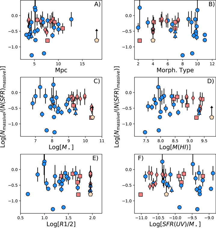
Figure 3. Panel A: ratio between the number of stars above 14 M⊙ as counted from the LEGUS data and the expected number of stars more massive than 14 M⊙ as derived from the measured SFRs as a function of distance (Panel A), morphological type (Panel B), total stellar mass (Panel C), mass of gas (Panel C), UV half-light radius (Panel E) and sSFR (Panel F). Spiral galaxies are marked in orange and dwarf galaxies are marked in blue. Spiral galaxies that fit within the WFC3 FoV are marked with square symbols, while spirals significantly larger than the WFC3 FoV are marked with diamonds. Similarly, dwarf galaxies that fit in the WFC3 FoV are indicated by circles, while dwarfs whose half-light radii are significantly larger than the WFC3's FoV are indicated by triangles. NGC 1566, for which we have only a lower limit, is indicated by a yellow pentagon.
Download figure:
Standard image High-resolution imageAs mentioned above, we assumed constant SFR over the past 100 Myr. While this assumption is probably correct for spiral and Magellanic galaxies, for the dwarf systems it is more likely that SF occurred in short bursts. Depending on when and at which rate SF developed in the dwarf galaxies, this can cause either an overestimation or an underestimation of the total number of massive stars. Panel A of Figure 3, for example, shows a correlation between the number of massive stars found in the field of dwarf galaxies and their distance. This trend is due to the fact that the majority of the late-type (RC3 T-type ≥8) dwarfs in the LEGUS sample are between 4 and 6 Mpc. In the case of the spiral galaxies, on the contrary, we do not notice any obvious trend with distance. We do not find any obvious correlation between the ratio Nmassive/N(SFR)massive and the other quantities mentioned above, therefore we conclude that our measurements are mostly free from these selection effects.
Panel A of Figure 4 shows the ratio Nmassive/N(SFR)massive as a function of ΣSFR. Again, we do not notice any obvious trend in this plot.
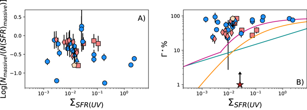
Figure 4. Panel A: ratio between the number of stars above 14 M⊙ as counted from the LEGUS data and the expected number of stars more massive than 14 M⊙ as derived from the measured SFRs as a function of  . Panel B: fraction of stars that likely formed in clustered environments as a function of
  . As in Figure 3, spiral galaxies are in orange and dwarf galaxies are in blue. Spiral galaxies that fit within the WFC3 FoV are marked with square symbols, while for spirals significantly larger than the WFC3 FoV we used diamond symbols. NGC 1566, for which we have only a lower limit, is marked with a yellow pentagon. Circles represent dwarf galaxies that fit within the WFC3 FoV, while larger dwarfs are indicated with triangles. The red stars in Panel B mark the two targets (IC 4247 and UGCA 281) whose number of stars counted in the field exceeds the number of stars expected from the SFR. Our data are compared to a fitted relation obtained from observational Gamma values (cyan line Goddard et al. 2010), and the analytical predictions for the values of Γ by (Kruijssen 2012, yellow line) and (Johnson et al. 2016, magenta line). Both predictions were derived assuming the same dependence of Γ on the gas surface density from Kruijssen 2012, but using different gas to SFR surface density conversions.
Download figure:
Standard image High-resolution imageWe now introduce a new value,

as the fraction of stars that are not in the field, and therefore are likely to be in clustered star-forming regions (including both compact bound clusters and unbound associations). Hence, we defined the above quantity as Γ⋆ rather than Γ, since the latter quantity usually refers to the fraction of stellar mass that is formed in bound clusters only.
We should note that since we measured both Nmassive and N(SFR)massive for the same massive stars, their number ratio is equivalent to the mass ratio. Our parameter, being derived from stars more massive than 14 M⊙, probes timescales shorter than 14 Myr, and is unlikely to measure only the fraction of stellar mass in bound systems. Rather, it is measuring the fraction of stellar mass that is included in all young clusters and associations. Still, because our derivation covers the same restricted age range for all the galaxies and regions considered, over the three orders of magnitude range of ΣSFR, it enables several considerations.
Both observations and models indicate that the fraction of star formation occurring in bound stellar clusters changes as a function of ΣSFR. To probe whether Γ⋆ scales similarly as Γ, in Panel B of Figure 4 we plot Γ⋆ as a function of ΣSFR. The plot includes the prediction by Kruijssen (2012, yellow line), a modified version of the Kruijssen model that takes into account the change in the slope of the relation between ΣSFR and Σgas (Johnson et al. 2016, magenta line), and an observational fit to the observed distributions in the Γ versus ΣSFR plane proposed by Goddard et al. (2010, cyan line). Although there is scatter in the value of Gamma at different ΣSFR, we assume that these models and fit identify the loci occupied by the formation efficiencies of bound-cluster populations as a function of the ΣSFR of the host galaxies.
From the right panel of Figure 4 we can readily see that:
- 1.The observed values of Γ⋆ cover almost one order of magnitude at the low end of our range of ΣSFR.
- 2.Most of the data are above the predictions of all the bound-cluster curves, with ∼14% points having Γ⋆ > 80%. This suggests that in these regions most of the stars form in clustered environments (either bound or unbound) and remain close to their siblings for at least the first 10–15 Myr.
- 3.For ΣSFR < 0.1, 50% of the points have Γ⋆ below 50%.
- 4.
- 5.Although there is a large scatter, the Γ⋆ values at ΣSFR < 0.01 are systematically higher than the predictions from the models.
- 6.Because Γ⋆ includes the fraction of both bound and unbound systems, this may indicate that the timescale required for association dissolution is longer than the usually adopted 10 Myr (Fall et al. 2005).
The uncertainties in the assumption of a constant SFR over the past 100 Myr are likely to be about a factor 3, which is smaller than the scatter in the Γ⋆ values for ΣSFR ≲ 0.1. Furthermore, some of the data with the lowest Γ⋆ values are regions within large galaxies, where we expect the star formation history to have remained relatively constant. Thus, at the low end of the ΣSFR values, the fraction of stars that are in clustered structures spans almost the full range of Γ⋆ values, from less than 20% to almost 100%. This scatter is unlikely to be due to spurious factors like distance dependency in our ability to resolve stars, since there is no dependency of Nmassive/N(SFR)massive on distance (Figure 3—Panel (A))).
Conversely, at the high end of the ΣSFR range, we observe a decrease in the scatter of Γ⋆. Although low number statistics may have an effect on this trend, it is still informative that all data are around or slightly above predictions from models. Furthermore, the scatter in Γ⋆ for ΣSFR ≳ 0.1 is about a factor of 30 lower than that for ΣSFR ≲ 0.1. This appears to indicate that high ΣSFR galaxies, when they form clusters, retain a higher fraction of bound systems, thus the fraction contributing to the field (i.e.,dissolving) is proportionally a smaller fraction of the total SFR.
Roughly, the models we report in the right panel of Figure 4 mark a lower boundary to the values of Γ⋆ that we measure, suggesting that stars form preferentially in clustered environments and remain confined within these compact (both bound and unbound) structures for the first ∼10–15 Myr. This result implies that Γ (cluster formation efficiency of bound cluster) derived using ages below ∼10 Myr and cluster catalogs based on the compactness of systems, as for the LEGUS survey, will always suffer from contamination of systems that are in reality unbound (e.g., Adamo et al. 2017). Indeed, Messa et al. (2018) reported that in M51 Γ was estimated in the age range 1–10 Myr, which is a factor of 3 higher than the Γ estimated in the age range 10–100 Myr, i.e., well within the scatter observed with our analysis of Γ⋆.
6. Summary and Conclusions
LEGUS (GO-13364, PI Calzetti) is a multiwavelength survey of 50 nearby star-forming galaxies. In this paper we presented the data reduction and the photometric analysis of the resolved stellar populations found in the galaxy fields. The stellar photometry was measured by PSF-fitting using the photometry package DOLPHOT by analyzing each filter independently.
As for all the HST Treasury programs, all the data collected by the LEGUS project were made immediately available to the astronomical community. To increase the legacy value of the project, ACS archival data in the filters B, V, and/or I have been aligned to the LEGUS data and can be downloaded from the LEGUS webpage.44 We are now releasing the astrophotometric catalogs for the resolved stellar populations. Cluster catalogs for most of the LEGUS galaxies are also becoming available (Adamo et al. 2017).
The NUV CMDs probe the stellar content of the LEGUS galaxies down to M ≲ 5–10, M⊙ (depending on the galaxy distance), with lookback times of several tens of Myr. At the optical wavelengths the lookback time is larger than at least one billion years. The LEGUS galaxies cover a broad range of metallicities and SFRs, with the larger systems showing evidence for metallicity and SFR gradients.
For most of the galaxies we were able to clearly identify the TRGBs and derive independent estimates of their distances. We used the metallicity and reddening derived by comparing the CMDs with PARSEC isochrones to estimate the number of stars more massive than M = 14 M⊙ in the NUV CMDs.
By comparing the number of stars more massive that 14 M⊙ found in the field of the galaxies with the expected number of massive stars inferred from the FUV SFR, we were able to estimate the fraction of massive stars found in clustered environments (bound star clusters + unbound stellar associations) at early ages (≤14 Myr). Our survey spans three orders of magnitude in SFR density and shows that at early ages (≤10–15 Myr) the formation efficiency of compact (bound and unbound) stellar systems (Γ⋆) remains above the predicted cluster formation efficiency of bound systems and does not depend on ΣSFR. We observe significantly more scatter in the Γ⋆ versus ΣSFR for ΣSFR ≲ 0.1 than observed for higher values. We suggest that the reduced scatter may be driven by the increase of star formation happening in bound clusters for increasing ΣSFR. The lack of relation between Γ⋆ and ΣSFR suggests that the timescale for the evaporation of unbound structures is comparable or longer than 10 Myr, thus Γ estimated with cluster catalogs relying only on the compactness of the systems will be overpredicted if limited to short age ranges (1–10 Myr), because of contamination by compact unbound associations.
We thank the referee Nate Bastian for the constructive suggestions that considerably improved the paper.
A.A. acknowledges partial support from the Swedish Royal Academy. G.A. acknowledges support from the Science and Technology Facilities Council (ST/L00075X/1 and ST/M503472/1). C.D. acknowledges funding from the FP7 ERC starting grant LOCALSTAR (no. 280104). M.F. acknowledges support by the Science and Technology Facilities Council (grant number ST/L00075X/1). D.A.G. kindly acknowledges financial support by the German Research Foundation (DFG) through program GO1659/3-2. These observations are associated with program # 13364. Support for program # 13364 was provided by NASA through a grant from the Space Telescope Science Institute. This work is based on observations obtained with the NASA/ESA Hubble Space Telescope, at the Space Telescope Science Institute, which is operated by the Association of Universities for Research in Astronomy, Inc., under NASA contract NAS 5-26555.
Facilities: HST (WFC3 - , ACS). -
Appendix:
Here we present the NUV and optical CMDs for all the galaxies studied in LEGUS.
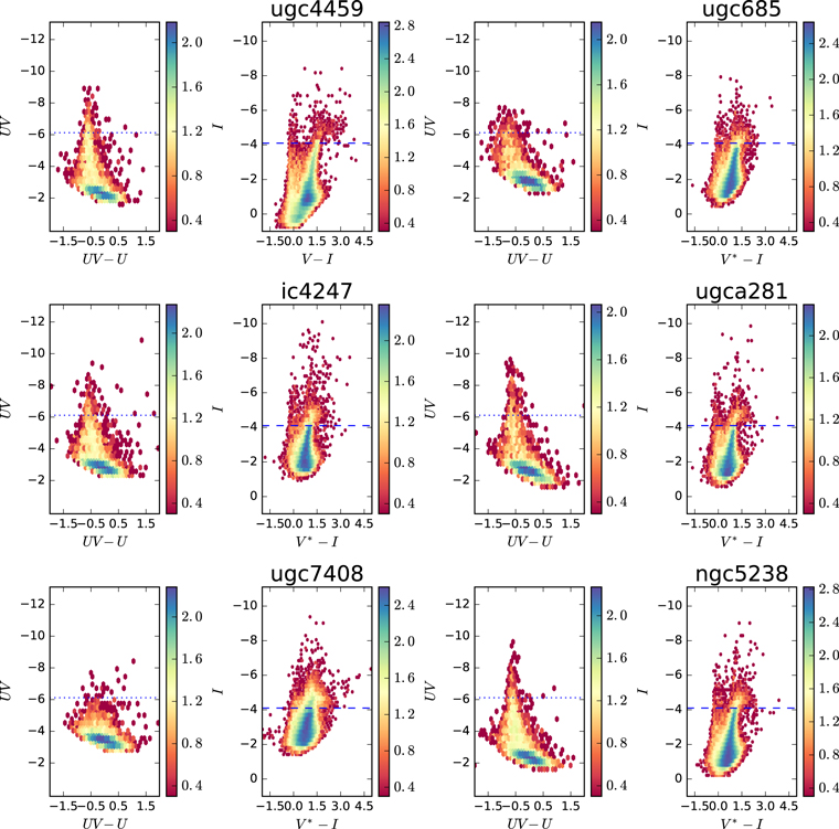
Figure 5. NUV and optical CMDs for the galaxies UGC 4459, UGC 685, IC4247, UGC A281, UGC 7408, and NGC 5238. Magnitudes marked as V* refer to the filter F606W, instead of F5555W.
Download figure:
Standard image High-resolution image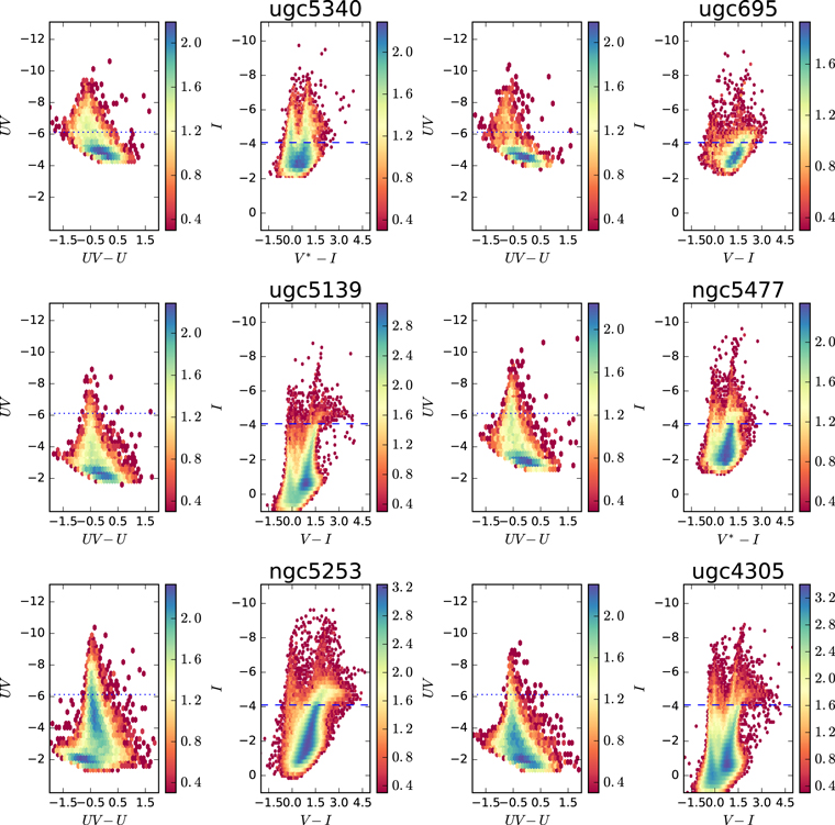
Figure 6. Same as Figure 5, but for the galaxies UGC 5340, UGC 695, UGC 5139, NGC 5477, NGC 5253, UGC 4305. Magnitudes marked as V* refer to the filter F606W, instead of F5555W.
Download figure:
Standard image High-resolution image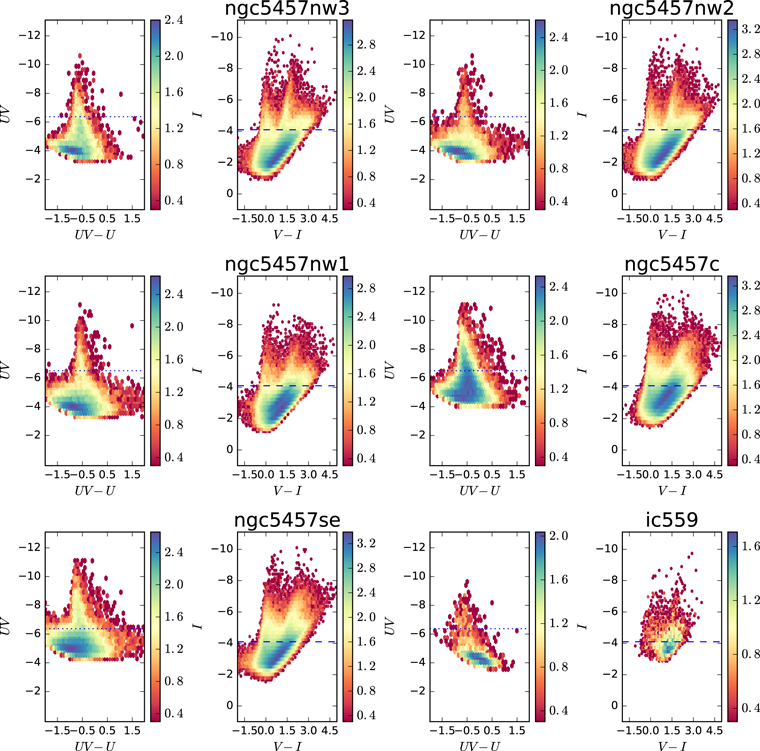
Figure 7. Same as Figure 5, but for the galaxy NGC 5457 (fields north west 3, north west 2, north west 1, center and south east), and the galaxy IC559.
Download figure:
Standard image High-resolution image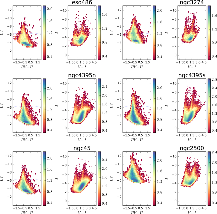
Figure 8. Same as Figure 5, but for the galaxies ESO486, NGC 3274, NGC 4395 (north and south), NGC 45, and NGC 2500.
Download figure:
Standard image High-resolution image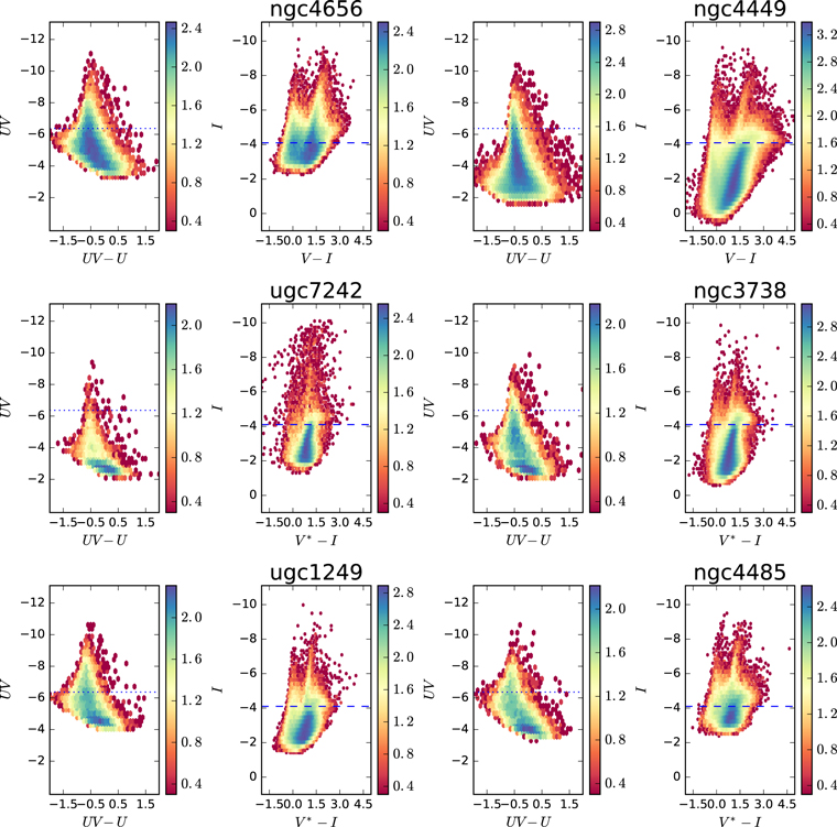
Figure 9. Same as Figure 5, but for the galaxies NGC 4656, NGC 4449, UGC 7242, NGC 3738, UGC 1249, NGC 4485. Magnitudes marked as V* refer to the filter F606W, instead of F5555W.
Download figure:
Standard image High-resolution image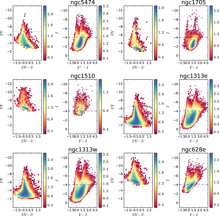
Figure 10. Same as Figure 5, but for the galaxies NGC 5474, NGC 1705, NGC 1510, NGC 1313 (east and west) and NGC 628 east. Magnitudes marked as V* refer to the filter F606W, instead of F5555W.
Download figure:
Standard image High-resolution image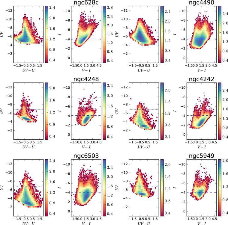
Figure 11. Same as Figure 5, but for the western part of the galaxies NGC 628 (west), NGC 4490, NGC 4248, NGC 4242, NGC 6503, and NGC 5949.
Download figure:
Standard image High-resolution image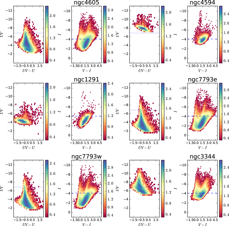
Figure 12. Same as Figure 5, but for the galaxies NGC 4605, NGC 4594, NGC 1291, NGC 7793 (east and west), and NGC 3344.
Download figure:
Standard image High-resolution image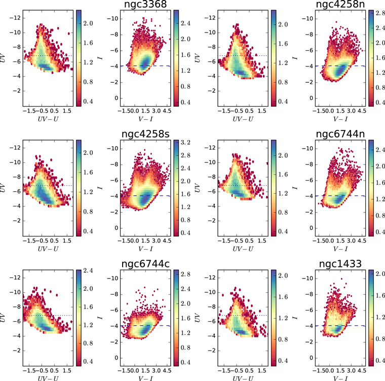
Figure 13. Same as Figure 5, but for the galaxies NGC 3368, NGC 4258 (north and south), NGC 6744 (north and Center), and NFC 1433.
Download figure:
Standard image High-resolution image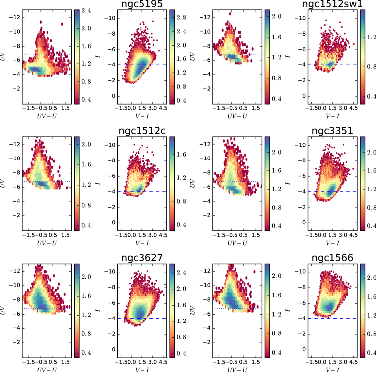
Figure 14. Same as Figure 5, but for the galaxies NGC 5195, NGC 1512 (southwest and Center), NGC 3351, NGC 3627, and NGC 1566.
Download figure:
Standard image High-resolution image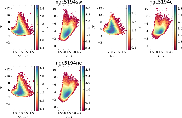
Figure 15. Same as Figure 5, but for the galaxy NGC 5194.
Download figure:
Standard image High-resolution imageFootnotes
- ∗
Based on observations with the NASA/ESA Hubble Space Telescope, obtained at the Space Telescope Science Institute, which is operated by AURA Inc., under NASA contract NAS 5-26555.
- 42
- 43
The CataPack package was developed by P. Montegriffo at the Bologna Observatory (INAF), and is available for download at http://www.bo.astro.it/~paolo/Main/CataPack.html.
- 44