Abstract
The Carnegie Supernova Project-II (CSP-II) was an NSF-funded, four-year program to obtain optical and near-infrared observations of a “Cosmology” sample of ∼100 Type Ia supernovae located in the smooth Hubble flow (0.03 ≲ z ≲ 0.10). Light curves were also obtained of a “Physics” sample composed of 90 nearby Type Ia supernovae at z ≤ 0.04 selected for near-infrared spectroscopic timeseries observations. The primary emphasis of the CSP-II is to use the combination of optical and near-infrared photometry to achieve a distance precision of better than 5%. In this paper, details of the supernova sample, the observational strategy, and the characteristics of the photometric data are provided. In a companion paper, the near-infrared spectroscopy component of the project is presented.
1. Introduction
A key goal of observational cosmology is to constrain the nature of dark energy through the detailed, accurate, and unbiased measurement of the expansion history of the universe. Einstein’s cosmological constant, for which the dark energy equation of state parameter, w, is precisely −1, is entirely consistent with the most recent results (Betoule et al. 2014; Scolnic et al. 2018); however, so are several competing models that are as fundamentally different from each other as they are to the cosmological constant (e.g., see the review by Yoo & Watanabe 2012). Currently, the tightest limits on the value of w come from combining observations of Type Ia supernovae (SNe Ia) with data from other probes, such as the cosmic microwave background and galaxy clustering. Excluding SNe Ia from these analyses results in considerably weaker constraints on w (e.g., Sullivan et al. 2011; Betoule et al. 2014). Nevertheless, the power of experiments such as the Baryon Oscillation Spectroscopic Survey (BOSS; Dawson et al. 2013) and its successor, the Dark Energy Spectroscopic Instrument (DESI; DESI Collaboration et al. 2016), to constrain w is expected to soon match and perhaps exceed the power of the current state-of-the-art SNe Ia experiments.
Improving the experiments with SNe Ia is not just a question of observing more SNe Ia, as any survey, no matter how large, will ultimately be limited by systematic errors related to both the photometric calibration and the physical nature of SNe Ia (e.g., Conley et al. 2011; Scolnic et al. 2018). In the optical, SNe Ia are not perfect standard candles. Rather, their successful use in cosmology is due to the discovery of empirical relations between luminosity, light-curve decline rate, and color that dramatically decrease the dispersion in peak luminosities (Pskovskii 1977; Phillips 1993; Tripp 1998). These relationships reduce the intrinsic Hubble diagram scatter typically to ∼0.15 mag (∼7% in distance). A luminosity correction dependent on host-galaxy mass has also been introduced (Kelly et al. 2010; Lampeitl et al. 2010; Sullivan et al. 2010). Recently, this effect has been confirmed by Uddin et al. (2017) using a sample of 1338 SNe Ia. Interestingly, those authors found that SNe Ia in hosts with high specific star formation rates display the lowest intrinsic dispersion (0.08 ± 0.01 mag) in luminosity after correction for light-curve decline rate and host-galaxy mass (see also Rigault et al. 2013).
Reducing the Hubble diagram scatter even further is highly desirable, as it directly leads to tighter cosmological constraints. However, at optical wavelengths, reducing the scatter has proved difficult, despite many years of effort. Fortunately, observations in the near-infrared (NIR) offer a way forward. This is because extinction from dust is reduced in the NIR, and because SNe Ia in the NIR are intrinsically better standard candles (Elias et al. 1985; Meikle 2000). NIR observations may also avoid possible dimming by dust in the intergalactic medium, currently only poorly constrained with optical observations (Goobar et al. 2018). The potential of SNe Ia as distance indicators in the NIR has been clearly demonstrated by Krisciunas et al. (2004b), Wood-Vasey et al. (2008), Mandel et al. (2011), Barone-Nugent et al. (2012), and (Stanishev et al. 2018), and by the extensive observations of the first phase of the Carnegie Supernova Project (CSP-I; Folatelli et al. 2010; Kattner et al. 2012; Phillips 2012; Burns et al. 2014, 2018).
The CSP-I was an NSF-funded project initiated in 2004 September to establish a fundamental data set of optical and NIR light curves of SNe Ia in a well-defined and understood photometric system (Hamuy et al. 2006). The CSP-I optical imaging was obtained over 1000 nights with the Las Campanas Observatory (LCO) Henrietta Swope 1 m telescope in the Sloan Digital Sky Survey ugri filters and Johnson BV filters. The NIR imaging was obtained with the Swope telescope and the LCO 2.5 m du Pont telescope, mostly in the YJH bandpasses. Over the five-year duration of the project, optical light curves were obtained for 123 SNe Ia, 83 SNe II, and 34 SNe Ib/Ic/IIb, with NIR photometry having been obtained for ∼85% of these. In addition, over 250 SNe of all types (including 129 SNe Ia) were monitored via optical spectroscopy. We have found that the data set for the Type Ia events has allowed us to improve dust-extinction corrections (Burns et al. 2014, 2018) and to investigate systematic effects in absolute magnitudes possibly due to differences in either age or metallicity, or both. The CSP-I observations are also being used to gain a deeper understanding of the physics of SNe Ia (e.g., Höflich et al. 2010; Hoeflich et al. 2017; Gall et al. 2018).
The CSP-I SN Ia optical and NIR light curves were published in three data release papers (Contreras et al. 2010; Stritzinger et al. 2011b; Krisciunas et al. 2017), and most of the optical spectra have also been published (Folatelli et al. 2013). In a recent paper by Burns et al. (2018), we have presented a full analysis of the uBgVriYJH Hubble diagrams for the CSP-I sample using new intrinsic color relations as a function of the sBV color-stretch parameter (Burns et al. 2014). Excluding the u band, which is affected by Ca ii H & K absorption features (Burns et al. 2014), we found peculiar-velocity-corrected dispersions of 5%–7% in distance for the full sample of 120 SNe, and 4%–6% for the subset of events with sBV > 0.5 and (B − V) < 0.5 mag. However, the median sample redshift of the CSP-I SNe Ia is z = 0.024, where the root mean square (rms) effect due to peculiar velocities is ∼4% in distance, and therefore is comparable to the intrinsic dispersion that we are attempting to measure. This limitation can be overcome by extending observations further into the smooth Hubble flow as shown by Barone-Nugent et al. (2012), who found a dispersion of 0.08 mag (a distance error of 4%) for a sample of a dozen SNe Ia that had redshifts 0.03 < z < 0.09. A similar result was obtained more recently by Stanishev et al. (2018) for a sample of 16 SNe Ia in the redshift range z = 0.037–0.183. Improving NIR K-corrections offers an additional refinement in precision because poorly understood K-corrections directly impact the peak magnitudes of the SNe and inflate both statistical and systematic errors (Boldt et al. 2014).
In 2011, we began a second phase of the Carnegie Supernova Project (CSP-II) to obtain optical and NIR observations of SNe Ia in the smooth Hubble flow. Over a four-year period, light curves were obtained for 214 SNe Ia at redshifts 0.004 < z < 0.137. NIR spectra were also obtained for 157 SNe Ia. This unique data set should provide an essential test of the ultimate precision of SNe Ia as distance indicators for determining the local value of the Hubble constant and constraining the nature of dark energy. The NIR spectra will also be a valuable resource for studying the physics and progenitors of SNe Ia (e.g., see Wheeler et al. 1998).
In this paper, details of the photometric portion of the CSP-II are presented. In Section 2, the CSP-II “Cosmology” and “Physics” SNe Ia subsamples are described in more detail, along with a third homogenous subsample discovered by the La Silla-QUEST (LSQ) supernova survey. Next, in Section 3, the observing strategy is presented. This is followed in Sections 4 and 5 with details of the photometric reductions. In Section 6, sample optical and NIR light curves representative of the full data set are given, followed by a summary of conclusions in Section 7.
2. Supernova Subsamples
The CSP-II covered four observing seasons spanning 7–8 months each and centered on the Chilean summer, beginning in 2011 October and ending in 2015 May. A final total of 214 SNe Ia was observed with redshifts in the range 0.004 < z < 0.137. Table 1 provides basic information for each SN including coordinates, host-galaxy identifications, and heliocentric redshifts. Also listed are the discovery programs from which the SNe were drawn and the sources of the classification spectra that identified these events as SNe Ia. In cases of multiple discoveries of the same SN, the name of the survey that first posted the discovery is listed first, and the SN is identified by the name given by the first discoverer. The horizontal lines in the table separate the SNe into the main survey groups (ASASSN, CRTS, KISS, LSQ, etc.).
Table 1. CSP-II SNe Ia
| SN Name | R.A. (2000) | Decl. (2000) | Host Galaxy | zhelioa | Discoveryb | Classificationb | Subsamplec |
|---|---|---|---|---|---|---|---|
| ASASSN-14ad | 12:40:11.10 | +18:03:32.80 | KUG 1237+183 | 0.0264 | ASASSN | (14) | P |
| ASASSN-14hp | 21:30:31.42 | −70:38:34.35 | 2MASX J21303015-7038489 | 0.0389 | ASASSN | CSP | C |
| ASASSN-14 hr | 01:50:41.27 | −14:31:06.37 | 2MASX J01504127-1431032 | 0.0336 | ASASSN | CSP | C |
| ASASSN-14hu | 06:43:26.92 | −69:38:14.70 | ESO 058- G 012 | 0.0216d | ASASSN | CSP | P |
| ASASSN-14jc | 07:35:35.29 | −62:46:12.64 | 2MASX J07353554-6246099 | 0.0113 | ASASSN | PESSTO | P |
| ASASSN-14jg | 23:33:13.90 | −60:34:11.50 | 2MASX J23331223-6034201 | 0.0148 | ASASSN | LCOGT | P |
| ASASSN-14jz | 18:44:44.34 | −52:48:05.48 | GALEXASC J184443.33-524819.2 | 0.0158d | ASASSN | PESSTO | |
| ASASSN-14kd | 22:53:24.95 | +04:47:57.30 | 2MASX J22532475+0447583 | 0.0242d | ASASSN | PESSTO | |
| ASASSN-14kq | 23:45:15.51 | −29:47:01.14 | 2MASX J23451480-2947009 | 0.0336 | ASASSN | CSP | C |
| ASASSN-14lo | 11:51:53.11 | +18:32:29.00 | UGC 06837 | 0.0199 | ASASSN | LCOGT | P |
| ASASSN-14lp | 12:45:09.10 | −00:27:32.49 | NGC 4666 | 0.0051 | ASASSN | ASASSN | P |
| ASASSN-14lq | 22:57:19.41 | −20:58:00.76 | 2MASX J22571481-2058014 | 0.0262 | ASASSN | (15) | P |
| ASASSN-14lt | 03:11:02.54 | −13:06:38.76 | IC 0299 | 0.0320 | ASASSN | Asiago | C |
| ASASSN-14lw | 01:06:49.17 | −46:58:59.96 | GALEXASC J010647.95-465904.1 | 0.0209d | ASASSN | CSP | P |
| ASASSN-14me | 01:26:40.08 | −57:59:49.31 | ESO 113- G 047 | 0.0178d | ASASSN | ASASSN | P |
| ASASSN-14mf | 00:04:54.46 | −32:26:14.63 | GALEXASC J000454.54-322615.3 | 0.0311 | ASASSN | ASASSN | C |
| ASASSN-14mw | 01:41:25.16 | −65:37:01.26 | AM 0139-655 NED02 | 0.0274 | ASASSN,OGLE | ASASSN | C,P |
| ASASSN-14my | 11:38:29.98 | −08:58:35.79 | NGC 3774 | 0.0205 | ASASSN,PS1 | CSP | P |
| ASASSN-15aj | 10:52:53.26 | −32:55:34.86 | NGC 3449 | 0.0109 | ASASSN | CSP | P |
| ASASSN-15al | 04:57:49.63 | −21:35:34.11 | GALEXASC J045749.46-213526.3 | 0.0338d | ASASSN,Gaia | PESSTO | C |
| ASASSN-15as | 09:39:16.55 | +06:25:48.53 | SDSS J093916.69+062551.1 | 0.0286d | ASASSN | CSP | C,P |
| ASASSN-15ba | 14:04:55.09 | +08:55:14.53 | SDSS J140455.12+085514.0 | 0.0231 | ASASSN,CRTS | CfA | P |
| ASASSN-15be | 02:52:46.39 | −34:18:52.52 | GALEXASC J025245.83-341850.6 | 0.0219 | ASASSN | ASASSN | P |
| ASASSN-15bm | 15:05:51.58 | −05:37:37.05 | LCRS B150313.2-052600 | 0.0208d | ASASSN | ASASSN | P |
| ASASSN-15cb | 12:39:50.23 | +03:47:49.77 | VCC 1810 | 0.0400 | ASASSN,PS1 | PESSTO | C |
| ASASSN-15 cd | 09 59 14.75 | +12 59 20.53 | CGCG 064-017 | 0.0344 | ASASSN | PESSTO | C |
| ASASSN-15 da | 05:23:51.88 | −24:42:08.38 | 2MASX J05235106-2442201 | 0.055e | ASASSN | ASASSN | C |
| ASASSN-15db | 15:46:58.69 | +17:53:02.55 | NGC 5996 | 0.0110 | ASASSN | (16) | |
| ASASSN-15dd | 15:43:59.07 | +19:12:40.74 | CGCG 107-031 | 0.0244 | ASASSN | ASASSN | |
| ASASSN-15eb | 08:06:07.40 | −22:33:48.86 | ESO 561- G 012 | 0.0165 | ASASSN | SMT | P |
| ASASSN-15fr | 09:20:20.44 | −07:38:26.78 | 2MASX J09202045-0738229 | 0.0334 | ASASSN | Asiago | C,P |
| ASASSN-15ga | 12:59:27.29 | +14:10:15.79 | NGC 4866 | 0.0066 | ASASSN | (17) | P |
| ASASSN-15go | 06:11:30.50 | −16:29:03.52 | 2MASX J06113048-1629085 | 0.0189 | ASASSN | SMT | P |
| ASASSN-15gr | 06:45:20.58 | −34:53:38.11 | ESO 366- G 015 | 0.0243d | ASASSN | PESSTO | P |
| ASASSN-15hf | 10:29:31.00 | −35:15:35.60 | ESO 375- G 041 | 0.0062 | ASASSN | PESSTO | P |
| ASASSN-15hg | 09:53:48.62 | +09:11:37.78 | CGCG 063-098 | 0.0298 | ASASSN | (18) | C |
| ASASSN-15hx | 13:43:16.69 | −31:33:21.55 | GALEXASC J134316.80-313318.2 | 0.0083d | ASASSN | PESSTO | P |
| PSN J13471211-2422171 | 13:47:12.11 | −24:22:17.10 | ESO 509- G 108 | 0.0199 | BOSS,ASASSN | CSP | P |
| SN2014ao | 08:34:33.32 | −02:32:36.10 | NGC 2615 | 0.0141 | LOSS,ASASSN | Asiago | P |
| SN2014I | 05:42:19.80 | −25:32:39.90 | ESO 487-G36 | 0.0300 | BOSS,ASASSN | SMT | C,P |
| SN2014eg | 02:45:09.27 | −55:44:16.90 | ESO 154- G 010 | 0.0186 | (1),ASASSN | PESSTO | P |
| CSS111231:145323+025743 (SN2011jt) | 14:53:23.01 | +02:57:43.10 | CGCG 048-051 | 0.0278 | CRTS | LOSS | P |
| CSS120224:145405+220541 (SN2012aq) | 14:54:05.13 | +22:05:40.60 | SDSS J145405.13+220540.7 | 0.052e | CRTS | Asiago | C |
| CSS120301:162036-102738 (SN2012ar) | 16:20:36.02 | −10:27:38.30 | 2MASX J16203650-1028061 | 0.0283 | CRTS | Asiago | C,P |
| CSS120325:123816-150632 | 12:38:16.19 | −15:06:32.15 | Anonymous | 0.0972d | CRTS | CRTS | C |
| CSS121114:090202+101800 | 09:02:02.34 | +10:18:00.10 | SDSS J090202.18+101759.7 | 0.0371 | CRTS | (19) | C |
| CSS130215:033841+101827 (SN2013ad) | 03:38:41.04 | +10:18:27.22 | Anonymous | 0.0363d | CRTS | CSP | C |
| CSS130303:105206-133424 | 10:52:06.06 | −13:34:24.70 | GALEXASC J105206.27-133420.2 | 0.0789d | CRTS | PESSTO | C |
| CSS130315:115252-185920 (SN2013as) | 11:52:52.34 | −18:59:19.90 | Anonymous | 0.0685d | CRTS | PESSTO | C |
| CSS131031:095508+064831 | 09:55:08.22 | +06:48:31.40 | SDSS J095510.00+064830.3 | 0.0777 | CRTS | PESSTO | C |
| CSS140126:120307-010132 | 12:03:06.88 | −01:01:31.70 | SDSS J120306.76-010132.4 | 0.0772d | CRTS | PESSTO | C |
| CSS140218:095739+123318 | 09:57:39.11 | +12:33:17.70 | SDSS J095738.31+123308.5 | 0.0773d | CRTS | PESSTO | C |
| CSS140914:010107-101840 | 01:01:07.04 | −10:18:39.90 | Anonymous | 0.03e | CRTS | PESSTO | C |
| CSS140925:162946+083831 (SN2014dl) | 16:29:46.09 | +08:38:30.60 | UGC 10414 | 0.0330 | CRTS | CSP | C |
| CSS150214:140955+173155 (SN2015bo) | 14:09:55.13 | +17:31:55.60 | NGC 5490 | 0.0162 | CRTS | PESSTO | P |
| SNhunt161 (SN2012hl) | 00:50:17.76 | +24:31:52.20 | CSS J005017.69+243154.4 | 0.0332d | CRTS | (20) | |
| SNhunt177 (SN2013az) | 05:39:52.13 | −40:30:28.10 | ESO 306-016 | 0.0373 | CRTS | PESSTO | C |
| SNhunt178 (SN2013bc) | 13:10:21.31 | −07:10:24.10 | IC 4209 | 0.0225 | CRTS | CSP | P |
| SNhunt188 (SN2013bz) | 13:26:51.32 | −10:01:32.20 | 2MASX J13265081-1001263 | 0.0192 | CRTS | (21) | P |
| SNhunt229 (SN2014D) | 12:10:36.76 | +18:49:35.40 | UGC 07170 | 0.0082 | CRTS,PS1 | CSP | P |
| SNhunt281 (SN2015bp) | 15:05:30.07 | +01:38:02.40 | NGC 5839 | 0.0041 | CRTS | (22) | P |
| SSS111226:125715-172401 (SN2011jn) | 12:57:14.79 | −17:24:00.50 | 2MASX J12571157-1724344 | 0.0475 | CRTS | (23) | C |
| MASTER OT J093953.18+165516.4 | 09:39:53.18 | +16:55:16.40 | CGCG 092-024 | 0.0478 | MASTER,CRTS | PESSTO | C |
| SN2014du | 02:26:23.31 | +27:39:34.80 | UGC 01899 | 0.0325 | ISSP,CRTS | Asiago | C,P |
| KISS13j (SN2013Y) | 12:09:39.70 | +16:12:14.30 | SDSS J120939.62+161212.2 | 0.0766 | KISS | KISS | C |
| KISS13l (SN2013al) | 11:14:54.07 | +29:35:06.00 | SDSS J111454.06+293508.7 | 0.1321 | KISS | (24) | C |
| KISS13v (SN2013ba) | 13:52:56.63 | +21:56:21.70 | SDSS J135256.58+215621.1 | 0.080e | KISS | KISS | C |
| KISS15m | 12:06:00.83 | +20:36:18.40 | NGC 4098 | 0.0243 | KISS,CRTS | CSP | |
| SN2015M | 13:00:32.33 | +27:58:41.00 | GALEXMSC J130032.33+275842.3 ? | 0.0231g | KISS,CRTS,PS1 | CSP | P |
| LSQ11bk | 04:20:44.25 | −08:35:55.75 | Anonymous | 0.0403d | LSQ | CSP | C,L |
| LSQ11ot | 05:15:48.34 | +06:46:39.36 | CGCG 421-013 | 0.0273 | LSQ | (25) | C,P,L |
| LSQ11pn (SN2011jq) | 05:16:41.54 | +06:29:29.40 | 2MASX J05164149+0629376 | 0.0327 | LSQ | SNF | C,P,L |
| LSQ12ca | 05:31:03.62 | −19:47:59.28 | 2MASX J05310364-1948063 | 0.0994d | LSQ | LCOGT | L |
| LSQ12agq | 10:17:41.67 | −07:24:54.45 | GALEXASC J101741.80-072452.2 | 0.0642d | LSQ | CSP | C,L |
| LSQ12aor | 10:55:17.64 | −14:18:01.38 | GALEXASC J105517.85-141757.2 | 0.0934d | LSQ | CSP | C,L |
| LSQ12bld | 13:42:44.03 | +08:05:33.74 | SDSS J134244.72+080531.7 | 0.0837 | LSQ | CSP | C,L |
| LSQ12blp | 13:36:05.59 | −11:37:16.87 | LCRS B133326.3-112212 | 0.0743 | LSQ,CRTS | CSP | C,L |
| LSQ12btn | 09:21:30.47 | −09:41:29.86 | 2MASX J09213114-0941331 | 0.0542 | LSQ | PESSTO | C,L |
| LSQ12cda | 13:50:02.32 | +09:37:47.10 | SDSS J135002.40+093755.1 | 0.1376 | LSQ | PESSTO | C,L |
| LSQ12cdl | 12:53:39.96 | −18:30:26.16 | GALEXASC J125339.85-183025.6 | 0.1081d | LSQ | PESSTO | C,L |
| LSQ12fuk | 04:58:15.88 | −16:17:58.03 | GALEXASC J045815.88-161800.7 | 0.0206d | LSQ,CRTS | SNF | P,L |
| LSQ12fvl | 05:00:50.04 | −38:39:11.51 | MCG -06-12-002 | 0.0560 | LSQ | PESSTO | C,L |
| LSQ12fxd | 05:22:17.02 | −25:35:47.01 | ESO 487- G 004 | 0.0312 | LSQ,CRTS | PESSTO | C,P,L |
| LSQ12gdj | 23:54:43.32 | −25:40:34.09 | ESO 472- G 007 | 0.0303 | LSQ | SNF | C,P,L |
| LSQ12gef | 01:40:33.70 | +18:30:36.38 | 2MASX J01403375+1830406 | 0.0642d | LSQ | SNF | L |
| LSQ12gln | 05:22:59.41 | −33:27:51.32 | GALEXASC J052259.58-332755.3 | 0.1021d | LSQ | PESSTO | C,L |
| LSQ12gpw | 03:12:58.24 | −11:42:40.13 | 2MASX J03125885-1142402 | 0.0506d | LSQ | PESSTO | L |
| LSQ12gxj | 02:52:57.38 | +01:36:24.25 | 2MASX J02525699+0136231 | 0.0355f | LSQ | PESSTO | L |
| LSQ12gyc | 02:45:50.07 | −17:55:45.74 | Anonymous | 0.0932f | LSQ | PESSTO | L |
| LSQ12gzm | 02:40:43.61 | −34:44:25.87 | GALEXASC J024043.58-344425.0 | 0.1001d | LSQ | PESSTO | L |
| LSQ12hjm | 03:10:28.72 | −16:29:37.08 | 2MASX J03102844-1629333 | 0.0714d | LSQ | SNF | L |
| LSQ12hno | 03:42:43.25 | −02:40:09.76 | GALEXASC J034243.43-024007.7 | 0.0473d | LSQ | CSP | C,L |
| LSQ12hnr | 10:43:14.77 | −08:46:40.89 | Anonymous | 0.135f | LSQ | PESSTO | C,L |
| LSQ12hvj | 11:07:38.62 | −29:42:40.96 | GALEXASC J110738.65-294235.5 | 0.0713d | LSQ | CSP | C,L |
| LSQ12hxx | 03:19:44.23 | −27:00:25.68 | 2MASX J03194423-2700201 | 0.0694 | LSQ | SNF | C,L |
| LSQ12hzj | 09:59:12.43 | −09:00:08.25 | 2MASX J09591230-0900095 | 0.0334d | LSQ | SNF | C,P,L |
| LSQ12hzs | 04:01:53.21 | −26:39:50.15 | 2MASXi J0401529-263947 | 0.0721 | LSQ | CSP | C,L |
| LSQ13lq | 13:44:10.81 | +03:03:43.42 | SDSS J134410.77+030345.3 | 0.0757d | LSQ | PESSTO | C,L |
| LSQ13pf | 13:48:14.35 | −11:38:38.58 | LCRS B134534.3-112338 | 0.0861d | LSQ | CSP | C,L |
| LSQ13ry | 10:32:48.00 | +04:11:51.75 | SDSS J103247.83+041145.5 | 0.0299 | LSQ | CSP | C,P,L |
| LSQ13vy | 16:06:55.85 | +03:00:15.23 | 2MASX J16065563+0300046 | 0.0418d | LSQ | LCOGT | C,L |
| LSQ13abo | 14:59:21.20 | −17:09:09.34 | 2MASX J14592124-1709138 | 0.0675 | LSQ | SNF | C,L |
| LSQ13aiz (SN2013cs) | 13:15:14.81 | −17:57:55.65 | ESO 576- G 017 | 0.0092 | LSQ,CRTS | (26) | P,L |
| LSQ13cwp | 04:03:50.65 | −02:39:17.98 | 2MASX J04035024-0239275 | 0.0666 | LSQ | CSP | C,L |
| LSQ13dby | 03:26:42.84 | −34:38:05.49 | Anonymous | 0.100e | LSQ | PESSTO | C,L |
| LSQ13dcy | 04:55:16.42 | −20:00:05.40 | LCSB S0801P | 0.0801d | LSQ | PESSTO | C,L |
| LSQ13dhj | 02:12:34.48 | −37:20:22.81 | GALEXMSC J021234.60-372019.1 | 0.0935d | LSQ | PESSTO | C,L |
| LSQ13dkp | 03:10:09.97 | −36:37:44.91 | 2MASX J03101094-3638017 | 0.0690 | LSQ | PESSTO | C,L |
| LSQ13dpm | 10:29:08.32 | −17:06:50.19 | GALEXASC J102908.61-170654.2 | 0.0509d | LSQ | PESSTO | C,L |
| LSQ13dqh | 04:22:05.90 | −02:53:24.24 | Anonymous | 0.1038d | LSQ | PESSTO | C,L |
| LSQ13dsm | 03:33:12.83 | −26:12:24.02 | APMUKS(BJ) B033105.19-262232.9 | 0.0424d | LSQ | CSP | C,L |
| LSQ14q | 08:53:57.58 | +17:19:38.19 | SDSS J085357.19+171942.6 | 0.0667 | LSQ,PS1 | PESSTO | C,L |
| LSQ14ba | 11:01:23.01 | −15:37:10.29 | GALEXASC J110123.17-153706.2 | 0.0776d | LSQ | PESSTO | C,L |
| LSQ14ie | 12:55:33.46 | −32:56:40.37 | Anonymous | 0.0896d | LSQ | PESSTO | C,L |
| LSQ14ip | 09:44:20.22 | +04:35:52.56 | 2MASX J09442084+0435319 | 0.0613 | LSQ | PESSTO | C,L |
| LSQ14jp | 12:57:21.51 | −15:47:33.42 | 2MASX J12572166-1547411 | 0.0454 | LSQ | CSP | C,L |
| LSQ14mc | 09:02:13.45 | +17:03:37.01 | SDSS J090213.35+170335.4 | 0.0567 | LSQ | PESSTO | C,L |
| LSQ14wp | 10:14:05.72 | +06:40:30.54 | SDSS J101405.83+064032.5 | 0.0695d | LSQ,CRTS | PESSTO | C,L |
| LSQ14xi | 12:30:41.17 | −13:46:21.91 | 2MASX J12304088-1346236 | 0.0508 | LSQ | PESSTO | C,L |
| LSQ14act | 15:59:44.65 | −10:26:40.80 | 2MASX J15594429-1026396 | 0.0591 | LSQ | PESSTO | C,L |
| LSQ14age | 13:24:08.62 | −13:26:26.00 | GALEXASC J132408.58-132629.0 | 0.0806d | LSQ | PESSTO | C,L |
| LSQ14ahc | 13:43:48.25 | −32:54:35.12 | 2MASX J13434760-3254381 | 0.0509d | LSQ | PESSTO | C,L |
| LSQ14ahm | 11:41:22.44 | −12:23:57.69 | GALEXASC J114122.65-122354.9 | 0.0498d | LSQ,CRTS | PESSTO | C,L |
| LSQ14ajn (SN2014ah) | 11:55:30.88 | +11:55:25.88 | CGCG 068-091 | 0.0210 | LSQ,PS1 | Asiago | P,L |
| LSQ14asu | 11:11:35.95 | −21:27:59.63 | 2MASX J11113635-2127597 | 0.0684 | LSQ | CSP | C,L |
| LSQ14auy | 14:28:11.30 | −04:03:17.50 | 2MASX J14281171-0403150 | 0.0825 | LSQ | CSP | C,L |
| LSQ14azy | 11:12:34.73 | +12:04:24.83 | 2MASX J11123493+1204206 | 0.0458 | LSQ | (27) | L |
| LSQ14bbv | 19:59:33.12 | −56:59:27.84 | 2MASS J19593264-5659334 | 0.0588d | LSQ | CSP | L |
| LSQ14bjj | 14:20:49.08 | −05:15:02.25 | APMUKS(BJ) B141811.91-050120.8 | 0.0812d | LSQ | PESSTO | C,L |
| LSQ14fms | 00:14:59.82 | −51:12:39.54 | 2MASX J00145929-5112380 | 0.078d | LSQ | CSP | C,L |
| LSQ14foj | 00:26:34.67 | −32:48:33.09 | GALEXASC J002634.59-324825.5 | 0.0461 | LSQ | PESSTO | C,L |
| LSQ14fom | 21:59:49.73 | −30:16:15.56 | 2MASX J21594968-3016187 | 0.0563 | LSQ | PESSTO | C,L |
| LSQ14gfb | 05:10:05.76 | −36:18:43.57 | 2MASX J05100559-3618388 | 0.0527 | LSQ | PESSTO | C,L |
| LSQ14gfn | 03:28:32.16 | −04:12:14.22 | 2MASX J03283205-0412113 | 0.1217d | LSQ | CSP | C,L |
| LSQ14ghv | 03:23:44.15 | −31:35:03.17 | 2MASX J03234449-3135101 | 0.0667 | LSQ | LCOGT | C,L |
| LSQ14gov | 04:06:01.33 | −16:01:41.49 | GALEXMSC J040601.67-160139.7 | 0.0896d | LSQ | PESSTO | C,L |
| LSQ15bv | 10:59:47.29 | −16:49:10.63 | 2MASX J10594717-1649070 | 0.0689 | LSQ | (28) | C,L |
| LSQ15aae | 16:30:15.70 | +05:55:58.73 | 2MASX J16301506+0555514 | 0.0516d | LSQ | CSP | C,L |
| LSQ15agh | 10:52:54.78 | +23:27:41.65 | 2MASX J10525434+2335518 | 0.0603 | LSQ | CSP | C,L |
| LSQ15aja | 17:03:08.92 | +12:27:41.65 | SDSS J170308.90+122741.5 | 0.0700d | LSQ | PESSTO | C,L |
| LSQ15alq | 13:09:18.56 | −25:52:20.24 | ESO 508- G 016 | 0.0471 | LSQ,PS1 | CSP | C,L |
| MASTER OT J030559.89+043238.2 | 03:05:59.89 | +04:32:38.20 | SDSS J030559.63+043246.0 | 0.0282d | MASTER | CfA | P |
| OGLE-2012-SN-040 | 06:07:01.59 | −69:21:17.10 | 2MASX J06070178-6921180 | 0.0147 | OGLE | PESSTO | |
| OGLE-2013-SN-015 | 02:02:21.56 | −65:44:08.66 | 2MASX J02022241-6544090 | 0.0890d | OGLE | CSP | C |
| OGLE-2013-SN-109 | 01:46:09.34 | −67:28:00.10 | 2MASX J01460987-6727579 | 0.0868d | OGLE | PESSTO | C |
| OGLE-2013-SN-118 | 05:14:47.50 | −66:50:29.10 | 2MASX J05144615-6650292 | 0.0750d | OGLE | PESSTO | C |
| OGLE-2013-SN-123 | 05:58:30.38 | −63:33:38.30 | 2MASX J05583036-6333386 | 0.0614d | OGLE | PESSTO | C |
| OGLE-2013-SN-126 | 04:19:47.21 | −63:43:22.04 | Anonymous | 0.0597d | OGLE | PESSTO | C |
| OGLE-2013-SN-148 | 06:38:06.97 | −75:43:37.21 | 2MASX J06380745-7543288 | 0.0404d | OGLE | PESSTO | C |
| OGLE-2014-SN-019 | 06:13:48.04 | −67:55:15.00 | 2MASX J06134795-6755146 | 0.0359 | OGLE | PESSTO | C |
| OGLE-2014-SN-021 | 05:48:23.49 | −66:47:29.70 | Anonymous | 0.0422d | OGLE | SMT | C |
| OGLE-2014-SN-107 | 00:42:28.75 | −64:45:51.00 | APMUKS(BJ) B004021.02-650219.5 | 0.0664d | OGLE | PESSTO | C |
| OGLE-2014-SN-141 | 05:37:18.64 | −75:43:17.00 | 2MASX J05371898-7543157 | 0.0625d | OGLE | PESSTO | C |
| SN 2015F | 07:36:15.76 | −69:30:23.00 | NGC 2442 | 0.0049 | (2),OGLE | PESSTO | P |
| PS1-13eao | 03:29:56.35 | −28:46:17.70 | ESO 418- G 007 | 0.0378 | PS1 | PESSTO | C |
| PS1-14ra | 14:41:28.44 | +09:25:58.70 | IC 1044 | 0.0281 | PS1 | PESSTO | C,P |
| PS1-14rx | 12:46:53.35 | +14:47:50.10 | SDSS J124653.32+144748.4 | 0.0666 | PS1 | PESSTO | C |
| PS1-14xw | 16:52:57.93 | +02:23:36.50 | NGC 6240 | 0.0245 | PS1 | PESSTO | |
| PS15sv | 16:13:11.74 | +01:35:31.10 | GALEXASC J161311.68+013532.2 | 0.0333d | PS1 | PESSTO | C,P |
| SN2013ct | 01:12:54.92 | +00:58:45.70 | NGC 428 | 0.0038 | BOSS,PS1 | CSP | P |
| SN2013gy | 03:42:16.88 | −04:43:18.48 | NGC 1418 | 0.0140 | LOSS,PS1,CRTS | Asiago | P |
| PTF11pbp (SN2011hb) | 23:27:55.52 | +08:46:45.00 | NGC 7674 | 0.0289 | PTF,CRTS | PTF | C,P |
| PTF11ppn | 21:35:21.93 | +26:56:04.70 | 2MASX J21352164+2656051 | 0.0673d | PTF | PTF | C |
| PTF11pra (SN2011hk) | 02:18:45.81 | −06:38:31.00 | NGC 881 | 0.0176 | PTF | PTF | |
| PTF11qnr (SN2011im) | 22:44:25.45 | −00:10:02.00 | NGC 7364 | 0.0162 | PTF | PTF | P |
| iPTF13ez | 12:09:51.30 | +19:47:15.70 | SDSS J120951.25+194716.5 | 0.0436 | iPTF | iPTF | C |
| iPTF13anh | 13:06:50.45 | +15:34:32.36 | SDSS J130650.44+153432.7 | 0.0614d | iPTF,CRTS | iPTF | C |
| iPTF13duj | 21:13:44.78 | +13:34:33.10 | NGC 7042 | 0.0170 | iPTF | LCOGT | P |
| iPTF13dwl | 21:16:49.05 | +12:00:50.80 | GALEXASC J211648.97+120052.8 | 0.0875d | iPTF | iPTF | C |
| iPTF13dym | 23:24:30.19 | +14:39:04.00 | SDSS J232430.20+143903.6 | 0.0422 | iPTF | iPTF | C |
| iPTF13ebh | 02:21:59.98 | +33:16:13.70 | NGC 0890 | 0.0133 | iPTF | CSP | P |
| iPTF13efe | 08:43:39.30 | +16:10:37.30 | SDSS J084339.26+161037.5 | 0.0751d | iPTF,CRTS | iPTF | C |
| iPTF14fpg (SN2014dk) | 00:28:12.00 | +07:09:43.50 | SDSS J002812.09+070940.0 | 0.034e | iPTF,PS1,CRTS | Asiago | C,P |
| iPTF14yw (SN2014aa) | 11:45:03.58 | +19:58:25.40 | NGC 3861 | 0.0170 | iPTF | Asiago | P |
| iPTF14w | 12:03:31.29 | +02:02:34.00 | UGC 07034 | 0.0189 | iPTF | Asiago | P |
| iPTF14uo | 13:18:57.69 | +09:42:40.30 | GALEXASC J131857.37+094244.0 | 0.0913d | iPTF | iPTF | C |
| iPTF14yy | 12:26:09.17 | +09:58:44.20 | SDSS J122608.78+095847.1 | 0.0431 | iPTF | iPTF | C |
| iPTF14aje | 15:25:12.07 | −01:48:51.50 | SDSS J152512.43-014840.1 | 0.0276 | iPTF | iPTF | C |
| iPTF14gnl | 00:23:48.33 | −03:51:27.90 | LCSB S0066P | 0.0537 | iPTF | iPTF | C |
| ROTSE3 J123935.1+163512 (SN2012G) | 12:39:35.10 | +16:35:11.90 | IC 0803 NED01 | 0.0258d | ROTSE-III,MASTER | (29) | P |
| SMT J03253351-5344190 | 03:25:33.51 | −53:44:19.00 | Anonymous | 0.0592d | SMT | SMT | C |
| SN 2011iv | 03:38:51.34 | −35:35:32.00 | NGC 1404 | 0.0065 | BOSS | (30) | P |
| SN2011iy | 13:08:58.38 | −15:31:04.00 | NGC 4984 | 0.0043 | (3) | (31) | P |
| SN2011jh | 12:47:14.42 | −10:03:47.30 | NGC 4682 | 0.0078 | (4) | Asiago | P |
| SN2012E | 02:33:22.79 | +09:35:05.60 | NGC 975 | 0.0203 | (5) | Asiago | P |
| SN2012U | 02:06:04.33 | −55:11:37.50 | ESO 153- G 020 | 0.0197 | BOSS | (32) | P |
| SN2012ah | 23:25:59.63 | −81:54:33.30 | NGC 7637 | 0.0124 | BOSS | (33) | P |
| SN2012bl | 20:23:55.28 | −48:21:17.30 | ESO 234-019 | 0.0187 | CHASE | (34) | P |
| SN2012bo | 12:50:45.23 | −14:16:08.50 | NGC 4726 | 0.0254 | (6) | Asiago | P |
| SN 2012fr | 03:33:36.10 | −36:07:34.00 | NGC 1365 | 0.0055 | TAROT | SMT | P |
| SN2012gm | 23:17:37.03 | +14:00:08.90 | NGC 7580 | 0.0148 | (7) | Asiago | P |
| SN2012hd | 01:14:07.46 | −32:39:07.70 | IC 1657 | 0.0120 | BOSS | PESSTO | P |
| SN2012hr | 06:21:38.46 | −59:42:50.60 | ESO 121- G 026 | 0.0076 | BOSS | CSP | P |
| SN 2012ht | 10:53:22.75 | +16:46:34.90 | NGC 3447 | 0.0036 | (8) | (8) | P |
| SN2012id | 04:42:41.14 | +18:34:59.70 | 2MASX J04424248+1835003 | 0.0157 | (9) | Asiago | P |
| SN2012ij | 11:40:15.84 | +17:27:22.20 | CGCG 097-050 | 0.0110 | TNTS | (35) | P |
| SN2013E | 10:00:05.52 | −34:14:01.30 | IC 2532 | 0.0094 | BOSS | CSP | P |
| SN2013H | 09:06:30.70 | −75:49:01.50 | ESO 036- G 019 | 0.0155 | BOSS | CSP | P |
| SN2013M | 13:59:56.68 | −37:51:49.40 | ESO 325- G 043 | 0.0350 | BOSS | (36) | C,P |
| SN2013U | 10:01:12.00 | +00:19:42.30 | CGCG 008-023 | 0.0345 | (10) | Asiago | C,P |
| SN2013aa | 14:32:33.88 | −44:13:27.80 | NGC 5643 | 0.0040 | BOSS | (37) | P |
| SN2013aj | 13:54:00.68 | −07:55:43.80 | NGC 5339 | 0.0091 | (11) | (11) | P |
| SN2013ay | 18:42:37.86 | −64:56:13.50 | IC 4745 | 0.0157 | CHASE | CSP | P |
| SN2013cg | 09:26:56.77 | −24:46:59.60 | NGC 2891 | 0.0080 | CHASE | (38) | P |
| SN2013fy | 21:37:27.12 | −47:01:54.80 | ESO 287- G 040 | 0.0309 | BOSS | PESSTO | C,P |
| SN2013fz | 04:23:46.44 | −51:35:46.30 | NGC 1578 | 0.0206 | BOSS | PESSTO | P |
| SN2013gv | 03:09:57.31 | +19:12:49.20 | IC 1890 | 0.0341 | (12) | Asiago | C,P |
| SN2013hh | 11:29:04.37 | +17:14:09.50 | UGC 06483 | 0.0130 | TAROT | SMT | P |
| SN2013hn | 13:48:59.17 | −30:17:26.50 | IC 4329 | 0.0151 | (13) | LCOGT | P |
| SN2014Z | 01:44:07.99 | −61:07:07.40 | ESO 114- G 004 | 0.0213 | BOSS | CSP | P |
| SN2014at | 21:46:14.82 | −46:31:21.10 | NGC7119 | 0.0322 | BOSS | PESSTO | C,P |
| SN2014ba | 22:55:01.97 | −39:39:34.50 | NGC 7410 | 0.0058 | BOSS | (39) | P |
| SN2014bz | 13:56:04.19 | −43:35:09.90 | 2MASX J13560316-4334319 | 0.0225 | TAROT | SMT | |
| SN2014dn | 04:17:54.27 | −56:36:45.20 | IC 2060 | 0.0222 | BOSS | CSP | |
Notes.
aHeliocentric redshift are from the NASA/IPAC Extragalactic Database (NED) unless otherwise indicated. bASASSN (Shappee et al. 2014; Holoien et al. 2017); Asiago (Tomasella et al. 2014); BOSS (http://bosssupernova.com/); CHASE (Pignata et al. 2009); CfA (https://www.cfa.harvard.edu/supernova//RecentSN.html); CRTS (Djorgovski et al. 2011); CSP (this paper); iPTF (Kulkarni 2013); ISSP (http://italiansupernovae.org/en/project/description.html); Gaia (Altavilla et al. 2012); KISS (Morokuma et al. 2014); LCOGT (Howell et al. 2014); LOSS (Filippenko et al. 2001); LSQ (Baltay et al. 2013); MASTER (Gorbovskoy et al. 2013); OGLE (Wyrzykowski et al. 2014); PESSTO (Smartt et al. 2015); PS1 (Kaiser et al. 2010; Scolnic et al. 2018); PTF (Law et al. 2009); ROTSE-III (Akerlof et al. 2003); SMT (Scalzo et al. 2017); SNF (Wood-Vasey et al. 2004); TAROT (Klotz et al. 2008); TNTS (Yao et al. 2015). cC = “Cosmology”; P = “Physics”; L = “LSQ”. dRedshift measured by CSP-II. eApproximate redshift derived from SN spectrum. fPeter Nugent (private communication). gRedshift of Coma Cluster.References. (1) Kangas et al. (2014); (2) Monard et al. (2015); (3) Itagaki et al. (2011); (4) Nakano et al. (2011); (5) Cox et al. (2012); (6) Itagaki et al. (2012); (7) Rich et al. (2012); (8) Nishiyama et al. (2012); (9) Yusa et al. (2012); (10) Gagliano et al. (2013);(11) Cortini et al. (2013); (12) Kiyota et al. (2013); (13) Kot et al. (2013); (14) Zhang et al. (2014) (15) Zhang & Wang (2014b); (16) Zhang & Wang (2015); (17) Piascik & Steele (2015); (18) Falco et al. (2015); (19) Graham et al. (2012); (20) Howerton et al. (2012); (21) Howerton et al. (2013); (22) Jha et al. (2015); (23) Foley & Fong (2011); (24) Tanaka et al. (2013); (25) Hadjiyska et al. (2011); (26) Walker et al. (2013); (27) Galbany et al. (2014); (28) Hodgkin et al. (2015); (29) Odewahn (2012); (30) Stritzinger et al. (2011a); Chen et al. (2011b); (31) Chen et al. (2011a); Yamanaka et al. (2011); (32) Anderson et al. (2012); (33) Dennefeld et al. (2012); (34) Prieto (2012); (35) Wang et al. (2013); (36) Parker et al. (2013a); (37) Parker et al. (2013b); (38) Pignata et al. (2013); (39) Milisavljevic et al. (2014).
We divide the full sample of 214 SNe Ia into three subsamples, as illustrated in Figure 1, and described in the remainder of this section.
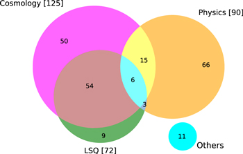
Figure 1. Venn diagram illustrating the subsamples into which the 214 SNe Ia observed by the CSP-II are divided. Note the significant overlap between the Cosmology, Physics, and LSQ subsamples.
Download figure:
Standard image High-resolution image2.1. Cosmology Subsample
The primary goal of the CSP-II was to obtain optical and NIR light curves of a sample of at least 100 SNe Ia located in the smooth Hubble flow out to a redshift of z ∼ 0.1. These SNe, which comprise the CSP-II “Cosmology” subsample, were selected for photometric follow-up via the following criteria:
- Discovered before maximum light at optical wavelengths. One of the few disadvantages of observing SNe Ia in the NIR is that maximum brightness occurs 3–5 days before B maximum. Hence, to ensure that NIR photometry was obtained within a few days of NIR maximum, SNe discovered before optical maximum light were given highest priority for follow-up observations.
- Spectroscopically confirmed to be a normal SNe Ia.27 Surveys such as the Sloan Digital Sky Survey-II Supernova Survey, the Supernova Legacy Survey (SNLS), and the Supernova Cosmology Project (SCP) have shown that combining magnitude and color information allows an “educated” guess to be made as to the SN type (Sako et al. 2011; Bazin et al. 2011; Suzuki et al. 2012). Nevertheless, spectroscopy is vital for confirmation purposes and determining the approximate light-curve phase, as well as for eventual sub-typing.
- Discovered preferably in an untargeted search. A weakness of the CSP-I SNe Ia sample is that nearly 90% of the events were found in targeted searches that are strongly biased toward luminous host galaxies (e.g., Kelly et al. 2010). Hence, for the CSP-II, preference was given to SNe Ia discovered in untargeted searches to ensure that the sample was as complete and unbiased as possible concerning host-galaxy type, luminosity, and metallicity.
- Host-galaxy redshift in the range 0.03 ≲ z ≲ 0.10. Many of the SNe Ia in the CSP-II Cosmology subsample appeared in host galaxies with cataloged redshifts. However, approximately one-third of the events were discovered in distant or low-luminosity hosts whose redshifts were unknown. In these cases, we relied on the redshift estimated from the classification spectrum with software tools such as SNID (Blondin & Tonry 2007), SUPERFIT (Howell et al. 2005), and GELATO (Harutyunyan et al. 2008) in deciding whether to obtain follow-up photometry. We have since obtained redshifts for nearly all of these host galaxies (see Section 3.6).
The 125 SNe Ia comprising the Cosmology subsample cover a redshift range of 0.027 < z < 0.137, with a median redshift of z = 0.056. Table 2 summarizes the various supernova surveys from which these SNe were drawn. Fully 96% came from untargeted searches, with nearly half (48%) of the subsample having been discovered by the La Silla-QUEST Low Redshift Supernova Survey (Baltay et al. 2013). The individual SNe belonging to the Cosmology subsample are identified in the final column of Table 1 by the letter “C”.
Table 2. CSP-II Cosmology Subsample Sources
| Source | Untargeted? | # of SNe | Percentage |
|---|---|---|---|
| LSQa | Yes | 60 | 48.0% |
| CRTSb | Yes | 15 | 12.0% |
| ASASSNc | Yes | 14 | 11.2% |
| PTF/iPTFd | Yes | 12 | 9.6% |
| OGLEe | Yes | 10 | 8.0% |
| PS1f | Yes | 4 | 3.2% |
| KISSg | Yes | 3 | 2.4% |
| SMTh | Yes | 1 | 0.8% |
| MASTERi | Yes | 1 | 0.8% |
| ⋯ | ⋯ | ||
| 120 | 96.0% | ||
| BOSSj | No | 3 | 2.4% |
| Otherl | No | 2 | 1.6% |
| ⋯ | ⋯ | ||
| 5 | 4.0% |
Notes.
aLa Silla-Quest Low Redshift Survey (Baltay et al. 2013). bCatalina Real Time Transit Survey (Djorgovski et al. 2011). cAll-Sky Automated Survey for SuperNovae (Shappee et al. 2014; Holoien et al. 2017). dPalomar Transient Factory (Law et al. 2009)/Intermediate Palomar Transient Factory (Kulkarni 2013). eOGLE-IV Real-Time Transient Search (Wyrzykowski et al. 2014). fPan-STARRS1 Medium Deep Survey (Kaiser et al. 2010; Scolnic et al. 2018). gKiso Supernova Survey (Morokuma et al. 2014). hSkyMapper Transient Survey (Scalzo et al. 2017). iMobile Astronomy System of TElescope Robots (Gorbovskoy et al. 2013). jBackyard Observatory Supernova Search http://bosssupernova.com/. kItalian Supernovae Search Project http://italiansupernovae.org/en/project/description.html. lGagliano et al. (2013); Kiyota et al. (2013).Download table as: ASCIITypeset image
The top panel of Figure 2 shows a histogram of the heliocentric redshifts of the Cosmology subsample. The arrow indicates the median redshift of the CSP-I sample. In Figure 3, histograms of the epoch with respect to the date of B maximum of the first imaging observations in the optical and the NIR for the Cosmology subsample are displayed. As may be seen, optical imaging was obtained for half of the subsample at −4 days or earlier, and −2 days or earlier in the NIR.
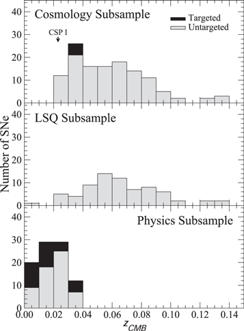
Figure 2. Top: histogram of heliocentric redshifts of the 125 SNe Ia comprising the Cosmology subsample. Bottom: the 90 SNe Ia in the Physics subsample. In the top panel, the median redshift of the CSP-I sample is indicated by an arrow. The middle panel displays a histogram of the redshifts of the LSQ subsample.
Download figure:
Standard image High-resolution image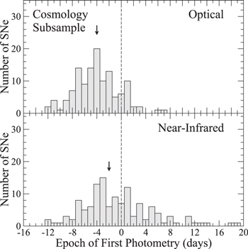
Figure 3. Top: histogram of the epoch with respect to the date of B maximum of the first optical imaging observations of the 125 SNe Ia comprising the Cosmology subsample. Bottom: similar histogram for the first NIR imaging observations. The arrows in each panel indicate the medians of the histograms corresponding to −4 days for the first optical photometry and −2 days for the first NIR observation.
Download figure:
Standard image High-resolution image2.2. Physics Subsample
To realize the full potential of SNe Ia as distance indicators at NIR wavelengths, we must determine accurate K-corrections, which account for the effect of cosmological expansion upon the measured magnitudes (Oke & Sandage 1968). Poorly understood K-corrections directly impact the peak magnitudes of the SNe and inflate both statistical and systematic errors. Prior to the CSP-II, NIR spectra had been published for only 33 SNe Ia, with the total number of useful spectra amounting to 75. Boldt et al. (2014) used this sample to study the errors inherent in NIR K-corrections. Their main finding was that uncertainties due to the diversity of spectral features from object to object are the dominant source of error at maximum light. Boldt et al. demonstrated that, with the small number of spectra in hand, K-correction uncertainties in the Y, J, and H bands amounted to 0.04, 0.06, and 0.10 mag for a SN Ia at z = 0.08. For a sample of 59 spectra of 10 SNe Ia—35 spectra of which overlapped with the Boldt et al. sample—Stanishev et al. (2018) recently found somewhat smaller dispersions of 0.03 and 0.04 mag in the J and H K-corrections at z = 0.08. Much of the diversity in the spectral features is known to correlate with the light-curve decline rate (Hsiao 2009), but to quantify this requires a much larger NIR spectral sample.
To attack the NIR K-correction problem, the CSP-II, in conjunction with the Harvard Center for Astrophysics Supernova Group, initiated in 2012 a program of NIR spectroscopic observations of a large “Physics” subsample28 of nearby SNe Ia at z ≤ 0.04. This collaboration is described in detail in an accompanying paper (Hsiao et al. 2018). In order to quantify the light-curve properties of this subsample, it was necessary to obtain optical imaging with a cadence and signal-to-noise ratio comparable to (or better than) that obtained for the Cosmology subsample. Although imaging in the NIR was not a requirement for the Physics subsample, it was nonetheless obtained for 89% of the SNe. The same basic criteria used for the Cosmology subsample were also applied in selecting the SNe to be included in the Physics subsample, although at these lower redshifts, a higher fraction (39%) of the events were discovered in targeted searches. The Physics subsample also includes several fast-declining, SN 1991bg-like (Filippenko et al. 1992a; Leibundgut et al. 1993; Ruiz-Lapuente et al. 1993) events that, because of their low luminosities, are not well represented in the Cosmology subsample.
A total of 90 SNe Ia with a median redshift of z = 0.021 comprise the Physics subsample. Table 3 provides information on the supernova surveys from which these SNe were drawn, and Table 1 lists the individual SNe (identified by the letter “P” in the final column). Their distribution as a function of redshift is plotted in the bottom panel of Figure 2. Note that there is some overlap between the Physics and Cosmology subsamples, with 21 of the SNe (23%) in the Physics subsample also forming part of the Cosmology subsample.
Table 3. CSP-II Physics Subsample Sources
| Source | Untargeted? | # of SNe | Percentage |
|---|---|---|---|
| ASASSNa | Yes | 27 | 30.0% |
| LSQb | Yes | 9 | 10.0% |
| CRTSc | Yes | 8 | 8.9% |
| PTF/iPTFd | Yes | 7 | 7.8% |
| PS1e | Yes | 4 | 4.4% |
| KISSf | Yes | 1 | 1.1% |
| MASTERg | Yes | 1 | 1.1% |
| OGLEh | Yes | 1 | 1.1% |
| ROTSE-IIIi | Yes | 1 | 1.1% |
| ⋯ | ⋯ | ||
| 59 | 65.6% | ||
| BOSSj | No | 14 | 15.6% |
| CHASEk | No | 3 | 3.3% |
| TAROTl | No | 2 | 2.2% |
| TNTSm | No | 1 | 1.1% |
| Othern | No | 11 | 12.2% |
| ⋯ | ⋯ | ||
| 31 | 34.4% |
Notes.
aAll-Sky Automated Survey for SuperNovae (Shappee et al. 2014; Holoien et al. 2017). bLa Silla-Quest Low Redshift Survey (Baltay et al. 2013). cCatalina Real Time Transit Survey (Djorgovski et al. 2011). dPalomar Transient Factory (Law et al. 2009)/Intermediate Palomar Transient Factory (Kulkarni 2013). ePan-STARRS1 Medium Deep Survey (Kaiser et al. 2010; Scolnic et al. 2018). fKiso Supernova Survey (Morokuma et al. 2014). gMobile Astronomy System of TElescope Robots (Gorbovskoy et al. 2013). hOGLE-IV Real-Time Transient Search (Wyrzykowski et al. 2014). iRobotic Optical Transient Search Experiment III (Akerlof et al. 2003). jBackyard Observatory Supernova Search http://bosssupernova.com/. kCHilean Automatic Supernova sEarch (Pignata et al. 2009). lTélescopes à Action Rapide pour les Objets Transitoires (Klotz et al. 2008). mTHU-NAOC Transient Survey (Zhang et al. 2015). nItagaki et al. (2011); Nakano et al. (2011); Cox et al. (2012); Itagaki et al. (2012); Rich et al. (2012); Nishiyama et al. (2012); Yusa et al. (2012); Gagliano et al. (2013); Cortini et al. (2013); Kiyota et al. (2013); Kot et al. (2013).Download table as: ASCIITypeset image
2.3. La Silla-QUEST Subsample
The La Silla-QUEST supernova survey was fundamental to the success of the CSP-II, contributing nearly half of the SNe Ia making up the Cosmology subsample. The LSQ subsample is particularly important because it was an untargeted search with homogeneous selection criteria. The recent dark energy analysis of the Pantheon sample of SNe Ia by Scolnic et al. (2018) found that systematic errors are still a serious problem, particularly in modeling the low-redshift sample because of the uncertainty of whether it is volume or magnitude limited. Calibration errors, which in the Pantheon sample are twice as large for the low-redshift events compared to the high-redshift SNe, also continue to be a significant additional source of systematic error. The LSQ subsample observed by the CSP-II addresses both of these issues.
The CSP-II obtained light curves of a total of 72 SNe Ia discovered by the LSQ survey, spanning a redshift range of 0.009 ≤ z ≤ 0.137. Preliminary photometry of 31 of these SNe was published by Walker et al. (2015). The LSQ subsample is identified in Table 1 by the letter “L” in the last column. Their redshift distribution is plotted in the middle panel of Figure 2. Note that 83% of the LSQ events are also members of the Cosmology subsample, and 13% overlap with the Physics subsample. NIR photometry was obtained for 85% of the LSQ subsample.
2.4. Other SNe Ia
Table 1 also includes 11 SNe Ia for which photometric observations were obtained, but which do not fit into any of the three aforementioned subsamples. These objects are identified by a blank entry in the “Subsample” column of the table. All have redshifts too small (z ≤ 0.026) to be included in the Cosmology subsample, and as NIR spectroscopy was not obtained they do not qualify for the Physics subsample. However, the light curves for these SNe are still of value, and so we include them in the full sample of CSP-II SNe Ia.
2.5. Other Types of SNe
The emphasis of the CSP-II was on observing the light curves and spectra of normal SNe Ia. Nevertheless, data were obtained for other types, including peculiar SNe Ia (five SN 2002cx-like events and four possible “super-Chandrasekhar” SNe), four super-luminous SNe, and several core-collapse and stripped core-collapse events. The CSP-II observations of these SNe will be presented in future papers.
3. Observing Strategy
3.1. Optical Imaging
As was the case for the CSP-I, nearly all of the optical imaging during the CSP-II was obtained with the LCO Swope telescope. Generally speaking, for redshifts less than ≲0.04, the same complement of ugriBV filters used by the CSP-I was also employed. For redshifts greater than this, a subset consisting of the BVri filters was normally used. Each SN was typically observed every 2–3 days from discovery until at least 2–3 weeks past maximum to sample the light-curve maxima and early decline rates as thoroughly as possible. Optical imaging of candidate SNe was often initiated before a classification spectrum was obtained. A quick reduction of the photometry was made the morning after each observation, allowing a nearly “real-time” update of the light curves on the CSP-II webpage, with the calibration improving as data were obtained on more photometric nights. If spectral observations subsequently showed that the target was not a SN Ia, we usually discontinued the optical imaging.
As was also done for the CSP-I, the LCO 2.5 m du Pont telescope was used to obtain most of the host-galaxy reference images in ugriBV. This telescope was also used to obtain a small amount of imaging of SNe being actively followed during scheduled nights.
3.2. NIR Imaging
SNe Ia are excellent standard candles in the NIR when observed at maximum light (e.g., Krisciunas et al. 2004a; Kattner et al. 2012). When combined with optical photometry, NIR observations at maximum also afford the most precise measurement of the host-galaxy dust reddening (Krisciunas et al. 2000; Mandel et al. 2011; Burns et al. 2014, 2018). While the strength of the prominent NIR secondary maximum is a strong function of the decline rate (Hamuy et al. 1996b), there is significant scatter in the correlation (Krisciunas et al. 2001; Burns et al. 2014). Hence, to ensure the highest precision for measuring both the host extinction and distance from optical and NIR observations, it is best that NIR photometry be obtained within ∼1 week of optical (B-band) maximum if at all possible (Krisciunas et al. 2004b). As shown in Figure 3, only a small fraction (11/125) of the SNe in the Cosmology subsample do not meet this condition.
The SNe in the CSP-I sample were sufficiently nearby and bright enough that all of the optical and most of the NIR imaging could be obtained with the Swope telescope. However, extending NIR observations to z ∼ 0.1 requires a larger telescope, and so a more economical approach was necessary for the CSP-II. We requested approximately one week of NIR imaging each bright run with the du Pont 2.5 m telescope during the CSP-II observing campaigns to cover the primary maxima of ∼5 SNe Ia per bright run. For SNe at z ≲ 0.07, imaging was generally obtained in the Y, J, and H bands, while for more distant targets, observations were typically restricted to the Y and J filters. In a few cases (<10%), only the Y filter was used. At least four epochs of NIR imaging were obtained for 66% of the SNe in the Cosmology subsample, and at least three epochs were obtained for 82%. Sparse sampling of the NIR maximum of SNe Ia has been successfully employed in the past by Krisciunas et al. (2004a); Freedman et al. (2009); Barone-Nugent et al. (2012), and Weyant et al. (2014, 2018).
Although most of the NIR photometry for the CSP-II was acquired with the du Pont telescope, we obtained a few epochs of additional imaging (1–2 epochs) with the LCO Magellan Baade 6.5 m telescope for nine SNe Ia. Many of the NIR host-galaxy images were also acquired with Magellan Baade.
3.3. Optical Spectroscopy
Optical spectroscopy near maximum light provides an essential tool for characterizing the diversity of SNe Ia which, in turn, is related to the progenitor systems and explosion mechanism (e.g., Blondin et al. 2012; Folatelli et al. 2013). In total, 308 optical spectra were obtained of more than 100 of the SNe Ia in the Cosmology and Physics subsamples. These spectra were acquired with the du Pont and Magellan telescopes at LCO and with the 2.5 m Nordic Optical Telescope (NOT) at the Observatorio del Roque de los Muchachos with the principal aim of determining the type, phase, and approximate redshift of the SN targets. Through these observations and the NIR spectroscopy described in Section 3.5 and Hsiao et al. (2018), the CSP-II was able to classify ∼20% of the SNe in both the Cosmology and Physics subsamples (listed as “CSP” in the Classification column of Table 1). Many of the remaining targets were classified by the Public ESO Spectroscopic Survey of Transient Objects (PESSTO) with the ESO La Silla 3.6 m NTT (Smartt et al. 2015). With the CSP-II, PESSTO, and other publicly available spectra, 114 of the SNe in the Cosmology and Physics subsamples were observed within ±4 days of maximum light. These data will be presented and analyzed in a future paper (N. Morrell et al., in preparation).
3.4. Optical Integral Field Spectroscopy
The pioneering work of the Calán/Tololo Project showed that SNe Ia luminosities are correlated with host-galaxy morphologies and colors (Hamuy et al. 1995, 1996a, 2000). More recently, evidence has been presented that SNe Ia Hubble diagram residuals correlate with global host-galaxy parameters such as total mass and star formation rate (Kelly et al. 2010; Lampeitl et al. 2010; Sullivan et al. 2010; Rigault et al. 2013; Uddin et al. 2017). To examine these effects for the CSP-II sample of SNe Ia, a program of integral field unit (IFU) host-galaxy spectroscopy is being carried out with both the Multi Unit Spectroscopic Explorer (MUSE) on the ESO VLT (Bacon et al. 2010) as part of the All-weather MUse Supernova Integral-field Nearby Galaxies (AMUSING) survey (Galbany et al. 2016), and the Potsdam Multi-Aperture Spectrophotometer (PMAS) on the 3.5 m Calar Alto telescope within the PMAS/PPak Integral-field Supernova hosts COmpilation (PISCO) program (Galbany et al. 2018) for those targets in the northern hemisphere. In addition to the global host properties, these IFU data will provide spectral information on the immediate environments of the SNe—e.g., line-of sight gas-phase and stellar metallicity, stellar age, and star formation rates—allowing a detailed study of the correlations between the SNe Ia Hubble diagram residuals and the local environmental properties.
3.5. NIR Spectroscopy
NIR spectroscopy was a new and vital component of the CSP-II. During the four campaigns, NIR spectra were obtained of 157 different SNe Ia. These observations were carried out using the Folded-port IR Echellette (FIRE) on the LCO Magellan Baade telescope and through target of opportunity (ToO) time obtained principally with the Gemini North and South 8.1 m telescopes, the NASA Infrared Telescope Facility (IRTF), and the ESO Very Large Telescope (VLT). This set of NIR spectra is more than 15 times larger than the previous largest sample (Marion et al. 2009). The FIRE spectra account for 80% of the total spectra obtained, but the ToO observations were crucial for obtaining spectral coverage at the earliest epochs. More than 70% of the SNe Ia observed have at least 3 epochs of NIR spectral observations, and more than 10 epochs were obtained for 15 SNe. Whenever possible, we also attempted to obtain simultaneous optical spectroscopy to match the NIR observations. The NIR spectroscopy part of the CSP-II is presented in detail in the accompanying paper by Hsiao et al. (2018).
3.6. Host-galaxy Redshifts
The majority of the SNe Ia in both the Cosmology and Physics subsamples were discovered in untargeted searches. Approximately one-third of the events selected for follow-up appeared in distant or low-luminosity hosts whose redshifts were unknown. A program of host-galaxy spectroscopy was initiated to measure redshifts for these SNe. Spectra of 40 of the hosts were obtained with the Wide-Field CCD (WFCCD) spectrograph on the du Pont telescope. For the faintest galaxies, it was necessary to use the Magellan telescopes. Spectra of 19 hosts were taken with the Inamori Magellan Areal Camera and Spectrograph (IMACS) on the Baade telescope, and another five galaxies were observed with the Low-Dispersion Survey Spectrograph (LDSS3-C) on the Clay telescope. Redshifts were obtained for an additional 11 host galaxies from our optical integral-field spectroscopy program.
The resulting redshifts are listed in Table 4, which gives the number of absorption and emission lines used to calculate the redshifts for each host-galaxy spectrum, and the rms errors of the final redshift values. These redshifts are also included in Table 1. Note that there are eight galaxies in Table 1 for which a redshift has not yet been measured.
Table 4. CSP-II Measurements of Host-galaxy Redshifts
| SN | Host Galaxy | Instrument(s)a | zHeliob | Linesc | |
|---|---|---|---|---|---|
| a | e | ||||
| ASASSN-14hu | ESO 058- G 012 | 1 | 0.0216 ± 0.0001 | 1 | 5 |
| ASASSN-14jz | GALEXASC J184443.33-524819.2 | 1 | 0.0158 ± 0.0001 | ⋯ | 8 |
| ASASSN-14kd | 2MASX J22532475+0447583 | 2 | 0.0242 ± 0.0002 | 1 | 3 |
| ASASSN-14lw | GALEXASC J010647.95-465904.1 | 2 | 0.0209 ± 0.0001 | ⋯ | 3 |
| ASASSN-14me | ESO 113- G 047 | 4 | 0.0178 ± 0.0001 | ⋯ | 5 |
| ASASSN-15al | GALEXASC J045749.46-213526.3 | 1 | 0.0338 ± 0.0001 | 2 | 3 |
| ASASSN-15as | SDSS J093916.69+062551.1 | 1 | 0.0286 ± 0.0001 | ⋯ | 3 |
| ASASSN-15bm | LCRS B150313.2-052600 | 1 | 0.0208 ± 0.0003 | 1 | 4 |
| ASASSN-15gr | ESO 366- G 015 | 1 | 0.0243 ± 0.0002 | ⋯ | 5 |
| ASASSN-15hx | GALEXASC J134316.80-313318.2 | 4 | 0.0083 ± 0.0002 | ⋯ | 4 |
| CSS120325:123816-150632 | Anonymous | 2 | 0.0972 ± 0.0002 | ⋯ | 5 |
| CSS130215:033841+101827 (SN2013ad) | Anonymous | 2 | 0.0363 ± 0.0001 | ⋯ | 4 |
| CSS130303:105206-133424 | GALEXASC J105206.27-133420.2 | 1 | 0.0789 ± 0.0004 | ⋯ | 1 |
| CSS130315:115252-185920 (SN2013as) | Anonymous | 1 | 0.0685 ± 0.0001 | ⋯ | 7 |
| CSS140126:120307-010132 | SDSS J120306.76-010132.4 | 2 | 0.0772 ± 0.0001 | ⋯ | 4 |
| CSS140218:095739+123318 | SDSS J095738.31+123308.5 | 2 | 0.0773 ± 0.0002 | ⋯ | 1 |
| LSQ11bk | Anonymous | 2 | 0.0403 ± 0.0001 | ⋯ | 5 |
| LSQ12ca | 2MASX J05310364-1948063 | 4 | 0.0994 ± 0.0003 | ⋯ | 3 |
| LSQ12agq | GALEXASC J101741.80-072452.2 | 3 | 0.0642 ± 0.0001 | ⋯ | 6 |
| LSQ12aor | GALEXASC J105517.85-141757.2 | 3 | 0.0934 ± 0.0001 | ⋯ | 8 |
| LSQ12cdl | GALEXASC J125339.85-183025.6 | 2 | 0.1081 ± 0.0001 | ⋯ | 6 |
| LSQ12fuk | GALEXASC J045815.88-161800.7 | 1 | 0.0206 ± 0.0002 | ⋯ | 4 |
| LSQ12gef | 2MASX J01403375+1830406 | 1 | 0.0642 ± 0.0004 | 6 | 3 |
| LSQ12gln | GALEXASC J052259.58-332755.3 | 3 | 0.1021 ± 0.0001 | ⋯ | 8 |
| LSQ12gpw | 2MASX J03125885-1142402 | 1 | 0.0506 ± 0.0002 | 1 | 4 |
| LSQ12gzm | GALEXASC J024043.58-344425.0 | 4 | 0.1001 ± 0.0002 | ⋯ | 5 |
| LSQ12hjm | 2MASX J03102844-1629333 | 1 | 0.0714 ± 0.0002 | 2 | 6 |
| LSQ12hno | GALEXASC J034243.43-024007.7 | 1 | 0.0473 ± 0.0001 | ⋯ | 7 |
| LSQ12hvj | GALEXASC J110738.65-294235.5 | 1 | 0.0713 ± 0.0001 | ⋯ | 4 |
| LSQ12hzj | 2MASX J09591230-0900095 | 2,4 | 0.0334 ± 0.0002 | 4 | ⋯ |
| LSQ13lq | SDSS J134410.77+030345.3 | 1 | 0.0757 ± 0.0002 | ⋯ | 4 |
| LSQ13pf | LCRS B134534.3-112338 | 2 | 0.0861 ± 0.0001 | 1 | 3 |
| LSQ13vy | 2MASX J16065563+0300046 | 1 | 0.0418 ± 0.0004 | 4 | 4 |
| LSQ13dcy | LCSB S0801P | 1,4 | 0.0801 ± 0.0003 | 7 | ⋯ |
| LSQ13dhj | GALEXMSC J021234.60-372019.1 | 1,4 | 0.0935 ± 0.0001 | ⋯ | 5 |
| LSQ13dpm | GALEXASC J102908.61-170654.2 | 1 | 0.0509 ± 0.0003 | ⋯ | 4 |
| LSQ13dqh | Anonymous | 2 | 0.1038 ± 0.0001 | ⋯ | 4 |
| LSQ13dsm | APMUKS(BJ) B033105.19-262232.9 | 1 | 0.0424 ± 0.0002 | ⋯ | 5 |
| LSQ14ba | GALEXASC J110123.17-153706.2 | 1 | 0.0776 ± 0.0001 | ⋯ | 4 |
| LSQ14ie | Anonymous | 1 | 0.0896 ± 0.0001 | ⋯ | 5 |
| LSQ14wp | SDSS J101405.83+064032.5 | 2 | 0.0695 ± 0.0001 | ⋯ | 4 |
| LSQ14age | GALEXASC J132408.58-132629.0 | 1 | 0.0806 ± 0.0003 | ⋯ | 5 |
| LSQ14ahc | 2MASX J13434760-3254381 | 2 | 0.0509 ± 0.0001 | ⋯ | 3 |
| LSQ14ahm | GALEXASC J114122.65-122354.9 | 1 | 0.0498 ± 0.0001 | ⋯ | 4 |
| LSQ14bbv | 2MASS J19593264-5659334 | 1 | 0.0588 ± 0.0006 | 7 | ⋯ |
| LSQ14bjj | APMUKS(BJ) B141811.91-050120.8 | 1 | 0.0812 ± 0.0001 | ⋯ | 7 |
| LSQ14fms | 2MASX J00145929-5112380 | 1 | 0.078 ± 0.001 | 3 | 2 |
| LSQ14gfn | 2MASX J03283205-0412113 | 2 | 0.1217 ± 0.0004 | 6 | ⋯ |
| LSQ14gov | GALEXMSC J040601.67-160139.7 | 1 | 0.0896 ± 0.0002 | ⋯ | 5 |
| LSQ15aae | 2MASX J16301506+0555514 | 1 | 0.0516 ± 0.0001 | 1 | 2 |
| LSQ15aja | SDSS J170308.90+122741.5 | 2 | 0.0700 ± 0.0001 | ⋯ | 4 |
| MASTER OT J030559.89+043238.2 | SDSS J030559.63+043246.0 | 1 | 0.0282 ± 0.0009 | ⋯ | 3 |
| OGLE-2013-SN-015 | 2MASX J02022241-6544090 | 1,4 | 0.0890 ± 0.0002 | 4 | ⋯ |
| OGLE-2013-SN-109 | 2MASX J01460987-6727579 | 1,4 | 0.0868 ± 0.0001 | ⋯ | 5 |
| OGLE-2013-SN-118 | 2MASX J05144615-6650292 | 1 | 0.0750 ± 0.0002 | ⋯ | 5 |
| OGLE-2013-SN-123 | 2MASX J05583036-6333386 | 1 | 0.0614 ± 0.0002 | 9 | ⋯ |
| OGLE-2013-SN-126 | Anonymous | 2 | 0.0597 ± 0.0002 | ⋯ | 3 |
| OGLE-2013-SN-148 | 2MASX J06380745-7543288 | 1 | 0.0404 ± 0.0002 | ⋯ | 6 |
| OGLE-2014-SN-021 | Anonymous | 3 | 0.0422 ± 0.0002 | ⋯ | 6 |
| OGLE-2014-SN-107 | APMUKS(BJ) B004021.02-650219.5 | 1 | 0.0664 ± 0.0001 | ⋯ | 3 |
| OGLE-2014-SN-141 | 2MASX J05371898-7543157 | 1 | 0.0625 ± 0.0002 | 1 | 8 |
| PS15sv | GALEXASC J161311.68+013532.2 | 1 | 0.0333 ± 0.0003 | ⋯ | 5 |
| PTF11ppn | 2MASX J21352164+2656051 | 1 | 0.0673 ± 0.0002 | 8 | ⋯ |
| iPTF13anh | SDSS J130650.44+153432.7 | 2 | 0.0614 ± 0.0001 | ⋯ | 6 |
| iPTF13dwl | GALEXASC J211648.97+120052.8 | 1 | 0.0875 ± 0.0002 | ⋯ | 6 |
| iPTF13efe | SDSS J084339.26+161037.5 | 2 | 0.0751 ± 0.0001 | ⋯ | 4 |
| iPTF14uo | GALEXASC J131857.37+094244.0 | 2 | 0.0913 ± 0.0001 | ⋯ | 7 |
| ROTSE3 J123935.1+163512 | IC 0803 NED01 (SN2012G) | 4 | 0.0258 ± 0.0002 | ⋯ | 5 |
| SMT J03253351-5344190 | Anonymous | 2,3 | 0.0592 ± 0.0002 | ⋯ | 5 |
| SNhunt161 (SN2012hl) | CSS J005017.69+243154.4 | 5 | 0.0332 ± 0.0002 | ⋯ | 6 |
Notes.
a1: du Pont+WFCCD, 2: Magellan Baade+IMACS, 3: Magellan Clay+LDSS3, 4: VLT+MUSE, 5: Calar Alto 3.5 m+PMAS/PPak. bThe heliocentric redshift measurement was derived from the equivalent-width-weighted average of the features listed in final column. A minimum error of 0.0001 is adopted from instrumental resolution considerations. cNumber of absorption (a) and emission (e) lines used to measure the redshift. Wavelengths of the features used to calculate the redshift are taken from Table 2 of Sandage (1978).4. Optical Photometry
4.1. Swope 1 m Telescope
As detailed in Krisciunas et al. (2017), the CSP-I employed the “SITe3” CCD camera and a set of Sloan Digital Sky Survey ugri and Johnson BV filters on the LCO Swope telescope to obtain optical light curves of the target SNe. The same setup was used for the first two campaigns of the CSP-II.29
However, for the third and fourth campaigns, the SITe3 camera was replaced with a new camera housing an e2V 4112 × 4096 pixel, deep depletion CCD with 15 μm pixels, four read-out amplifiers, and a two-layer anti-etalon, anti-reflection coating. At the focal plane of the Swope telescope, this corresponds to a 30′ × 30′ field with 0435 pixels. This is a larger field than was required for the CSP-II observations, so we used only quadrant 3 of the detector since it had the best linearity characteristics.
The relative throughputs of the ugriBV passbands with the new e2V CCD were measured in 2013 October using a monochromator and calibrated detectors (Rheault et al. 2014). As expected, the quantum efficiency of the e2V CCD was found to be more uniform and sensitive, both in the blue and the red, than the SITe3 CCD. The response functions (telescope + filter + CCD camera + atmosphere) for the SITe3 camera are plotted in cyan in Figure 4. These are based on measurements made at the telescope in 2010 January and July using the same monochromator (see Stritzinger et al. 2011b for the calibration details). Plotted in red in Figure 4 are the response functions for the e2V camera. The curves for both detectors have been normalized using the r band. The B, g, V, and i filters with the e2V CCD show increased sensitivity compared to the r filter than was the case with the SITe3 detector.
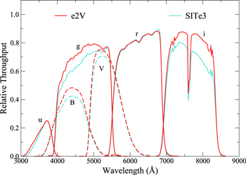
Figure 4. Cyan: optical filter response functions for the Swope telescope and SITe3 CCD camera used during the first two campaigns of the CSP-II. This is the same system used during the CSP-I. Red: optical filter response functions for the Swope telescope and e2V CCD camera used during the final two campaigns of the CSP-II. The B and V curves are plotted with dashed lines to aid in their discrimination. Note that the curves give the total relative throughput (telescope + filter + CCD camera + atmosphere) for an airmass of 1.2.
Download figure:
Standard image High-resolution imageThe methodology of the CSP photometric reductions is explained in detail in Krisciunas et al. (2017), but we briefly reproduce it here for completeness. First, we solve for color terms and extinction based on observations on photometric nights of Landolt (1992) and Smith et al. (2002) standard stars. We then fit the instrumental magnitudes, ugribv, via the following equations:






where u’g′r’i′BV correspond to magnitudes in the standard system, kλ are the extinction coefficients, X is the airmass, λ are the color terms, and ζλ are the zero-points. During the CSP-I project, ∼10 standard stars were observed per photometric night to determine the extinction and color terms. These were found to be highly stable over five years (see Figures 4 and 5 of Krisciunas et al. 2017). Hence, a slightly different calibration strategy was implemented for the CSP-II. The number of standard stars observed per night was decreased to ∼4–5, but standard-star observations were taken on as many clear nights as possible. As a result, data for determining extinction and color terms were obtained on considerably more nights during the CSP-II compared to the CSP-I.
Figure 5 displays the evolution of the nightly values of the zero-points during the CSP-II. As mentioned above, the detector in use for the first two years was the same SITe3 CCD used during the CSP-I. The significant jump in sensitivity at the end of year 2 is due to two nearly equal effects. The first is the washing of the primary mirror (indicated by the vertical gray dashed line), and the second is the higher quantum efficiency of the e2v CCD, which was put into operation immediately following the mirror washing. Each of these effects separately appears to have produced an increase in sensitivity of ∼50%. The steady decline in sensitivity observed for both detectors is due to the accumulation of dust and aerosols, principally on the primary mirror. The periodic dips in sensitivity correspond to the Chilean midsummer and most likely are due to an increase in atmospheric haze that is typical at this time of the year (Krisciunas et al. 2017).
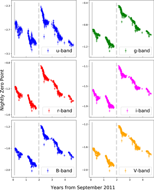
Figure 5. Nightly photometric zero-points derived from observations of local standard stars observed on clear nights with the LCO Swope telescope during the four years of the CSP-II. The solid vertical gray line corresponds to when the primary mirror of the telescope was aluminized; the dashed vertical gray line indicates when the primary mirror was washed, and also when the SITe3 detector was replaced by an e2v CCD. The few points falling below the general trend correspond to nights that appeared cloudless, but were not photometric. See the text for further details.
Download figure:
Standard image High-resolution imageTable 5 compares the final mean extinction and color coefficients for the Swope+e2V system with those of the Swope+SITe3. As was observed for the CSP-I (Krisciunas et al. 2017), the extinction terms were remarkably consistent during the four years of the CSP-II, testifying to the photometric stability of the atmosphere above LCO. As expected, some small differences are observed between the color coefficients, with the largest changes being in the blue (the u and B filters) and the red (the i filter).
Table 5. Optical Photometric Reduction Terms: SITe3 versus e2V
| Filter | Swope+SITe3 | Swope+e2V |
|---|---|---|
| Extinction Coefficientsa | ||
| u | 0.511 ± 0.057 | 0.509 ± 0.060 |
| B | 0.242 ± 0.022 | 0.233 ± 0.027 |
| g | 0.191 ± 0.021 | 0.186 ± 0.027 |
| V | 0.144 ± 0.018 | 0.135 ± 0.026 |
| r | 0.103 ± 0.019 | 0.094 ± 0.022 |
| i | 0.059 ± 0.020 | 0.057 ± 0.020 |
| Color Termsb | ||
| u | 0.046 ± 0.017 | 0.030 ± 0.020 |
| B | 0.061 ± 0.012 | 0.091 ± 0.015 |
| g | −0.014 ± 0.011 | −0.005 ± 0.014 |
| V | −0.058 ± 0.011 | −0.062 ± 0.015 |
| r | −0.016 ± 0.015 | −0.001 ± 0.022 |
| i | −0.002 ± 0.015 | 0.021 ± 0.018 |
Notes.
aMeasured in magnitudes per airmass. All uncertainties in this table are the “standard deviations of the distributions,” not the standard deviations of the means. bSee Equations (1)–(6) for which standard colors are used in combination with these coefficients to obtain the color correction terms for the optical photometry.Download table as: ASCIITypeset image
To measure final light curves for the SNe, we first established local sequence stars in each of the SN fields from observations of Landolt (1992) and Smith et al. (2002) standard stars. The underlying host-galaxy light was then subtracted from each SN image using host-galaxy reference images acquired after the SN had disappeared. These images were obtained mostly with the SITe2 CCD imager on the du Pont telescope. However, reference images for a number of SNe were acquired with the SITe3 CCD on the Swope telescope in good seeing (<1″) conditions. Magnitudes for the SN were then measured differentially with respect to the local sequence stars using point-spread-function (PSF) photometry (for further details, see Krisciunas et al. 2017). As a matter of policy, the CSP has been publishing all of its optical (and NIR) light curves in the natural photometric system of each telescope/instrument/filter combination, which is the “purest” form of the data (see Section 5.1 of Krisciunas et al. 2017).
4.2. du Pont 2.5 m Telescope
The LCO du Pont 2.5 m telescope was used with the facility Tek5 CCD camera to obtain host-galaxy reference images as well as a small amount of SN follow-up photometry. As discussed in detail in Section 6.1.2 of Krisciunas et al. (2017), experiments carried out on two SN fields observed in both the Swope SITe3 and du Pont+Tek5 systems confirm that the SN photometry obtained in the ugriBV filters with the du Pont+Tek5 is on substantially the same natural system as the Swope+SITe3 camera.
5. NIR Photometry
5.1. du Pont 2.5 m Telescope
NIR imaging in the YJH filters of the CSP-II SNe was obtained with RetroCam on the du Pont telescope. RetroCam employs a Rockwell 1024 × 1024 HAWAII-1 HgCdTe array with 18.5 μm pixels. This is the same NIR imager used at the Swope telescope during the CSP-I.30
RetroCam on the du Pont telescope gives a field of 34 × 3
4 and a pixel size of 0
201. For host galaxies that were larger than the dither pattern, separate sky images were obtained.
In 2013 October, Rheault et al. (2014) made spectrophotometric measurements of the RetroCam YJH bandpasses on the du Pont telescope, which can be compared with similar data collected in 2010 January with the same monochrometer when RetroCam was on the Swope telescope (Krisciunas et al. 2017). This is shown in Figure 6, where the total relative throughputs (telescope + filter + camera + atmosphere) are shown for RetroCam on the Swope and du Pont telescopes. As may be seen, the transmission functions of the Y and J bands did not change significantly between the two measurements. The most significant difference is in the H filter and is likely ascribed to variations in either or both of the reflective and transmissive properties of the optics of the two telescopes. Most importantly, for all three bandpasses, the filter edges have not shifted significantly in wavelength.
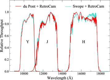
Figure 6. Cyan: YJH filter response functions for the LCO Swope telescope and RetroCam imager used during the CSP-I; Red: the LCO du Pont 2.5 m telescope and RetroCam used for NIR imaging during the CSP-II. Note that the curves give the total relative throughputs (telescope + filter + camera + atmosphere) for an airmass of ∼1.2.
Download figure:
Standard image High-resolution imageThe NIR imaging of the SNe was calibrated to local sequence stars established in the fields of each of the SNe. Calibration of the local sequence stars was carried out through observations on photometric nights of ∼4–5 of the Persson et al. (1998) standard stars. In analogy to the optical filters, the photometric transformation equations for the measured instrumental magnitudes, yjh, are



where kλ are the extinction coefficients, X is the airmass, λ are the color terms, and ζλ are the zero-points. In these equations, Jstd and Hstd are the magnitudes given in Persson et al. (1998), and Ystd is the magnitude in the RetroCam Y-band standard system defined by Krisciunas et al. (2017).
Zero-points derived from RetroCam during the 4+ years of the CSP-II are plotted in Figure 7. Note that these do not show the steady decline in sensitivity observed for the CCD detectors on the Swope telescope (cf. Figure 5). This is likely because the primary mirror of the du Pont telescope is cleaned with CO2 on an approximately weekly basis, whereas the closed-tube design of the Swope telescope does not permit this.
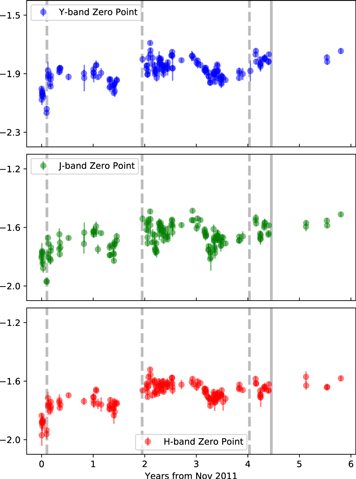
Figure 7. Nightly photometric zero-points derived from observations of standard stars observed on clear nights with RetroCam on the LCO 2.5 m du Pont telescope during the four years of the CSP-II. The dashed vertical gray lines indicate when the primary mirror was washed, and the solid vertical line corresponds to when the primary mirror was aluminized.
Download figure:
Standard image High-resolution imageExtinction coefficients in the Y, J, and H filters for RetroCam on the du Pont telescope were derived through a simultaneous Markov chain Monte Carlo fitting in the mixture model framework (Hogg et al. 2010) of all the CSP-II RetroCam nights. This procedure assumes a unique free parameter for the extinction coefficient, a fixed value of the color term estimated from synthetic photometry of model stellar atmospheres (see below), and the nightly zero point values. The resulting values are given in the top half of Table 6. We note that these differ slightly from the extinction coefficients measured with RetroCam on the Swope telescope during the CSP-I, but fall within the dispersion of the latter values (see Figure 8 of Krisciunas et al. 2017).
Table 6. NIR Photometric Reduction Terms
| Filter | du Pont+RetroCam | Baade+FourStar |
|---|---|---|
| Extinction Coefficientsa | ||
| Y | 0.069 ± 0.006 | … |
| J | 0.101 ± 0.006 | … |
| H | 0.056 ± 0.007 | … |
| Color Termsb | ||
| Y | 0.000 | 0.106 |
| J | 0.019 | 0.001 |
| H | −0.039 | −0.040 |
Notes.
aMeasured in magnitudes per airmass. Uncertainties in the extinction coefficients are the “standard deviations of the distributions,” not the standard deviations of the means. bSee Equations (7)–(9) for which standard colors are used in combination with these coefficients to obtain the color correction terms for the NIR photometry. The color terms in this table are estimated from synthetic photometry of Castelli & Kurucz (2003) stellar atmosphere models. The extinction coefficients measured for the du Pont+RetroCam were assumed for Baade+FourStar.Download table as: ASCIITypeset image
The NIR color terms could not be measured at the telescope due to the small color range, +0.19 ≤ (J − H) ≤ +0.35 mag, of the Persson et al. (1998) standard stars employed for the nightly photometric calibration. However, as we have precise spectrophotometric measurements of the NIR filter bandpasses, color terms can be estimated from synthetic photometry of model stellar atmospheres. This was done for the RetroCam JRC2 and H filters on the du Pont telescope in Appendix C of Krisciunas et al. (2017), and the resulting values, reproduced in Table 6, were shown to be consistent with observations made of the red stars listed in Table 3 of Persson et al. (1998). As expected from the close agreement of the RetroCam Y filter bandpasses on the Swope and du Pont telescopes (see Figure 6), the color term for this filter is negligible since the standard system is defined to be the natural system of RetroCam on the Swope telescope (Krisciunas et al. 2017).
Final measurement of the SN light curves was carried out in an analogous way to the optical photometry. Local sequence stars were established in each of the SN fields and magnitudes for the SNe were measured differentially with respect to these.
5.2. Magellan Baade 6.5 m Telescope
Host-galaxy reference images were obtained mostly with the FourStar imager (Persson et al. 2013) on the Magellan Baade telescope, due to the superior throughput and image quality of this instrument. (Some reference images were also obtained with RetroCam on the du Pont telescope on nights of excellent seeing.) As mentioned in Section 3.2, a few active SNe were also observed with FourStar. FourStar employs four HAWAII-2RG detectors that cover a 108 × 10
8 field of view with a pixel scale of 0
159. Filter response functions for the FourStar filters are illustrated in Figure 8. Note that FourStar does not have a Y filter, but the J1 filter provides a useful alternative. When imaging CSP-II SNe, the target was centered typically in chip 2. If the host galaxy was larger than the dither pattern, the target was alternately positioned in chip 2 and chip 4 to construct sky images in both chips.
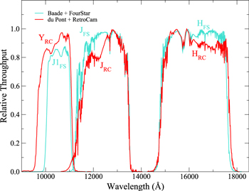
Figure 8. Filter response functions for the Baade telescope and FourStar imager. The FourStar filters are plotted in cyan and are compared with the du Pont + RetroCam filters, which are plotted in red. FourStar does not have a Y filter, but the J1 filter provides a reasonable approximation (see Contreras et al. 2018). Note that the filter curves give the total relative throughputs (telescope + filter + camera + atmosphere) for an airmass of ∼1.2.
Download figure:
Standard image High-resolution imageThe Persson et al. (1998) red stars are far too bright to be observed with FourStar on the Magellan Baade telescope, and so we must also estimate the color terms for this instrument from synthetic photometry of model atmospheres. The resulting values are listed in Table 6.
6. First Results
Figure 9 displays optical and NIR light curves of four SNe Ia in the Cosmology subsample observed during the first CSP-II campaign. These objects were selected as representative of both the range of data quality and redshifts covered by the subsample. The photometric measurements have been fitted with the SuperNovae in object oriented Python (SNooPy; Burns et al. 2011) package.
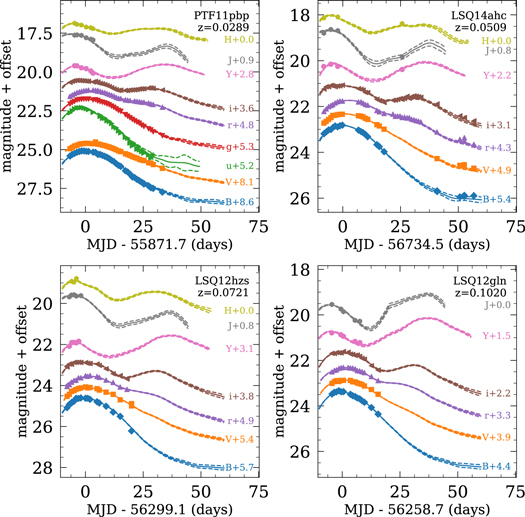
Figure 9. Light curves of four representative SNe Ia (PTF11pbp, LSQ14ahc, LSQ12hzs, and LSQ12gln) are plotted with offsets for clarity. In most cases, the error bars representing the statistical uncertainties are smaller than the symbols. The data have been fitted using the “max_model” option in SNooPy (Burns et al. 2011) which fits the maximum magnitude in each filter using a template generator based on well-observed optical and NIR light curves from the CSP-I The solid lines represent SNooPy fits to each filter’s light curve, while the dashed lines represent the ±1σ errors in the light-curve templates. The filter names and magnitude offsets are labeled to the right of each light curve.
Download figure:
Standard image High-resolution imageIn the left panel of Figure 10, histograms of the B-band decline rate, Δm15(B), of the SNe Ia in the Cosmology and Physics subsamples are plotted as determined from the SNooPy template fits. In the right panel of this figure, histograms of the color-stretch parameter, sBV (Burns et al. 2014), are also plotted. The distribution of the decline-rate parameters for the two subsamples differs only slightly in that the Physics subsample has relatively more fast decliners (smaller stretch). This may be due to that fact that 34% of the SNe Ia in the Physics subsample come from targeted searches monitoring predominately massive galaxies, where the vast majority of the fast decliners are found.
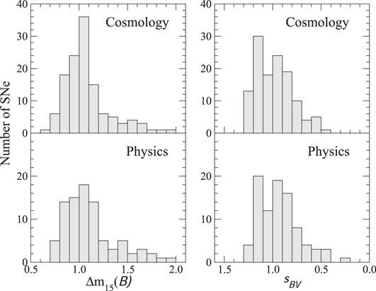
Figure 10. Histograms of the B-band decline-rate parameter, Δm15(B) (left panel), and the color-stretch parameter, sBV (right panel) for the Cosmology and Physics subsamples.
Download figure:
Standard image High-resolution imageThe final photometry data release for the full CSP-II sample of 214 SNe Ia is planned for 2019. Note that light curves and spectra for a few individual objects observed by the CSP-II have already been published: LSQ12gdj, a slow-declining, UV-bright SN Ia (Scalzo et al. 2014); iPTF13ebh, a transitional SN Ia showing strong NIR C i lines (Hsiao et al. 2015); SN 2011iv, a transitional SN Ia that was discovered in the same Fornax cluster galaxy that hosted SN 2007on, another transitional SN Ia observed during the CSP-I (Gall et al. 2018); SN 2012fr, a nearby, peculiar SN Ia observed within a day of explosion (Childress et al. 2013; Contreras et al. 2018); ASASSN-14lp, a bright SN Ia also discovered within two days of outburst (Shappee et al. 2016); SN 2012Z,a luminous SN Iax (Stritzinger et al. 2015); and SN 2013by, a Type IIL SN with a sharp light-curve decline after a short, steep plateau/linear decline phase (Valenti et al. 2015). Optical and NIR photometry of two SNe Ia observed by the CSP-II, SN 2012ht and SN 2015F, that appeared in host galaxies with Cepheid distances is presented in Burns et al. (2018).
7. Conclusions
This paper has presented a summary of the second phase of the Carnegie Supernova Project, which was carried out between 2011–2015. Photometry was obtained for a total of 214 SNe Ia with host-galaxy redshifts in the range 0.004 < z < 0.137. A “Cosmology” subsample of 125 SNe with both optical and NIR light curves at a median redshift of z = 0.056 is described. These SNe, along with the subsample of 72 SNe Ia discovered by the La Silla-QUEST survey, will be used to study the intrinsic precision of SNe Ia as cosmological distance indicators and to measure the local value of the Hubble constant. Light curves and NIR spectroscopy were also obtained of a second “Physics” subsample of 90 SNe Ia at a median redshift of z = 0.021. This subsample will be used to determine precise NIR K-corrections and to study the explosion physics and progenitors of SNe Ia. The 214 SNe Ia monitored by the CSP-II combined with the 123 SNe Ia observed during the CSP-I (Krisciunas et al. 2017) constitutes a sample of more than 300 SNe Ia with precise light curves in a well-understood photometric system. This data set will provide a definitive low-redshift reference for future rest frame optical and NIR observations of SNe Ia at high redshift with next-generation dark energy experiments such as the Euclid and WFIRST missions, and the LSST Dark Energy Science Collaboration.
The work of the CSP-II has been generously supported by the National Science Foundation under grants AST-1008343, AST-1613426, AST-1613455, and AST-1613472. The CSP-II was also supported in part by the Danish Agency for Science and Technology and Innovation through a Sapere Aude Level 2 grant. M. Stritzinger acknowledges funding by a research grant (13261) from VILLUM FONDEN. T. D. is supported by an appointment to the NASA Postdoctoral Program at the Goddard Space Flight Center, administered by Universities Space Research Association under contract with NASA.
Facilities: Magellan:Baade (IMACS imaging spectrograph - , FourStar wide-field near-infrared camera - , FIRE near-infrared echellette) - , Magellan:Clay (LDSS3 imaging spectrograph) - , Swope (SITe3 CCD imager - , e2v 4 K × 4 K CCD imager) - , du Pont (Tek5 CCD imager - , WFCCD imaging spectrograph - , RetroCam near-infrared imager) - , Gemini:North (GNIRS near-infrared spectrograph) - , Gemini:South (FLAMINGOS2) - , VLT (ISAAC - , MUSE) - , IRTF (SpeX near-infrared spectrograph) - , NOT (ALFOSC) - , Calar Alto 3.5 m (PMAS/PPak) - , La Silla-QUEST - , CRTS - , PTF - , iPTF - , OGLE - , ASAS-SN - , PS1 - , KISS - , ISSP - , MASTER - , SMT). -
Software: SNID (Blondin & Tonry 2007), SUPERFIT (Howell et al. 2005), GELATO (Harutyunyan et al. 2008), SNooPy (Burns et al. 2011).
Footnotes
- ∗
This paper includes data gathered with the 6.5 meter Magellan telescopes at Las Campanas Observatory, Chile.
- 27
In this paper, “normal” SNe Ia are defined to include “Branch-normal” events (Branch et al. 1993), as well as the 1991T-like (Filippenko et al. 1992b; Phillips et al. 1992) and “transitional” (Hsiao et al. 2015) events which, while considered by some as extreme, nevertheless fall on the luminosity versus decline-rate relation for SNe Ia (Burns et al. 2018).
- 28
We choose to refer to these SNe as the “Physics” subsample because, as described in detail in Hsiao et al. (2018), the NIR spectral data are also an invaluable resource for studying the physics and the progenitors of SNe Ia.
- 29
All of the V-band images taken during the CSP-II were obtained with the “V(LC-3009)” filter (see Section 6.1.1 of Krisciunas et al. 2017 for more details).
- 30
Note that all of the RetroCam J-band observations made during the CSP-II were obtained with the “JRC2” filter (see Section 6.2.1 of Krisciunas et al. 2017 for more details).