ABSTRACT
We present improved synthesis models of the evolving spectrum of the UV/X-ray diffuse background, updating and extending our previous results. Five new main components are added to our radiative transfer code CUBA: (1) the sawtooth modulation of the background intensity from resonant line absorption in the Lyman series of cosmic hydrogen and helium; (2) the X-ray emission from the obscured and unobscured quasars that gives origin to the X-ray background; (3) a piecewise parameterization of the distribution in redshift and column density of intergalactic absorbers that fits recent measurements of the mean free path of 1 ryd photons; (4) an accurate treatment of the photoionization structure of absorbers, which enters in the calculation of the helium continuum opacity and recombination emissivity; and (5) the UV emission from star-forming galaxies at all redshifts. We provide tables of the predicted H i and He ii photoionization and photoheating rates for use, e.g., in cosmological hydrodynamics simulations of the Lyα forest and a new metallicity-dependent calibration to the UV luminosity density-star formation rate density relation. A “minimal cosmic reionization model” is also presented in which the galaxy UV emissivity traces recent determinations of the cosmic history of star formation, the luminosity-weighted escape fraction of hydrogen-ionizing radiation increases rapidly with look-back time, the clumping factor of the high-redshift intergalactic medium evolves following the results of hydrodynamic simulations, and Population III stars and miniquasars make a negligible contribution to the metagalactic flux. The model provides a good fit to the hydrogen-ionization rates inferred from flux decrement and proximity effect measurements, predicts that cosmological H ii (He iii) regions overlap at redshift 6.7 (2.8), and yields an optical depth to Thomson scattering, τes = 0.084 that is in agreement with Wilkinson Microwave Anisotropy Probe results. Our new background intensities and spectra are sensitive to a number of poorly determined input parameters and suffer from various degeneracies. Their predictive power should be constantly tested against new observations. We are therefore making our redshift-dependent UV/X emissivities and CUBA outputs freely available for public use at http://www.ucolick.org/~pmadau/CUBA.
1. INTRODUCTION
The reionization of the all-pervading intergalactic medium (IGM) is a landmark event in the history of cosmological structure formation. Studies of Gunn–Peterson absorption in the spectra of distant quasars show that hydrogen is highly photoionized out to redshift z ≳ 6 (e.g., Fan et al. 2006a; Songaila 2004), while polarization data from the Wilkinson Microwave Anisotropy Probe (WMAP) constrain the redshift of a sudden reionization event to be significantly higher, z = 10.5 ± 1.2 (Jarosik et al. 2011). It is generally thought that the IGM is kept ionized by the integrated UV emission from active nuclei and star-forming galaxies, but the relative contributions of these sources as a function of epoch are poorly known. Because of the high ionization threshold (54.4 eV) and small photoionization cross section of He ii, and of the rapid recombination rate of He iii, the double ionization of helium is expected to be completed by hard UV-emitting quasars around the peak of their activity at z ≈ 2.5 (e.g., Madau & Meiksin 1994; Sokasian et al. 2002; McQuinn et al. 2009), much later than the reionization of H i and He i. At z > 3, the declining population of bright quasars appears to make an increasingly small contribution to the 1 ryd radiation background, and it is believed that massive stars in galactic and subgalactic systems may provide the additional ionizing flux needed at early times (e.g., Madau et al. 1999; Gnedin 2000; Haehnelt et al. 2001; Wyithe & Loeb 2003; Meiksin 2005; Trac & Cen 2007; Faucher-Giguère et al. 2008a; Gilmore et al. 2009; Robertson et al. 2010). This idea may be supported by the detection of escaping ionizing radiation from individual Lyman break galaxies at z ∼ 3 (e.g., Shapley et al. 2006).
Despite much recent progress, a coherent description of the thermal state and ionization degree of the IGM remains elusive. The intensity and spectrum of the cosmic ultraviolet background remain one of the most uncertain yet critically important astrophysical input parameters for cosmological simulations of the IGM and for interpreting quasar absorption-line data and derive information on the distribution of primordial baryons (traced by H i, He i, He ii transitions) and of the nucleosynthetic products of star formation (C iii, C iv, Si iii, Si iv, O vi, etc.). This is the fourth paper in a series aimed at a detailed study of the generation and reprocessing of photoionizing radiation in a clumpy universe, and of the transfer of energy from this diffuse background flux to the IGM. In Paper I (Madau 1995) we showed how the stochastic attenuation produced by neutral hydrogen along the line of sight affects the colors of distant galaxies. In Paper II (Haardt & Madau 1996) we developed CUBA, a radiative transfer code that followed the propagation of Lyman-continuum (LyC) photons through a partially ionized inhomogeneous IGM. CUBA outputs have been extensively used to model the Lyα forest in large cosmological simulations (e.g., Tytler et al. 2004; Theuns et al. 1998; Davé et al. 1997; Zhang et al. 1997). In Paper III (Madau et al. 1999) we focused on the candidate sources of photoionization at early times and on the history of the transition from a neutral IGM to one that is almost fully ionized. In this paper, we describe a new version of CUBA and use it to compute improved synthesis models of the UV/X-ray cosmic background spectrum and evolution, combining, updating, and extending many of our previous results in this field. The five main upgrades to CUBA are: (1) the sawtooth modulation from resonant line absorption in the Lyman series of intergalactic helium as well as hydrogen; (2) the X-ray emissivity from the obscured and unobscured populations of active galactic nuclei (AGNs) that gives origin to the X-ray background (XRB); (3) an up-to-date piecewise parameterization of the distribution in column density of intervening absorbers, which establishes the “super Lyman-limit systems” (SLLSs) as the dominant contributors to the hydrogen LyC intergalactic opacity; (4) an accurate treatment of the absorber photoionization structure, entering in the calculation of the helium continuum opacity and recombination emissivity of the clumpy IGM; and (5) the UV flux from star-forming galaxies at all redshifts.
The plan is as follows. In Section 2, we review the basic theory of cosmological radiative transfer in a clumpy universe. Sections 3 and 4 discuss the distribution of absorbers along the line of sight and their photoionization structure. The recombination radiation from the clumpy IGM is calculated in Section 5. In Sections 6 and 7 we compute the UV and X-ray emissivity from quasars, and in Section 8 the UV emissivity from star-forming galaxies. An overview of the main results generated by the updated CUBA radiative transfer code is given in Section 9. Finally, we summarize our findings in Section 10. Unless otherwise stated, all results shown below will assume a  cosmology. Note that, while the source volume emissivities must be evaluated in a given cosmological model, the resulting background intensity does not explicitly depend on the choice of cosmological parameters.
2. COSMOLOGICAL RADIATIVE TRANSFER
We start by summarizing the basic theory describing the propagation of ionizing radiation in a clumpy, primordial IGM (e.g., Paper I; Paper II; Madau & Haardt 2009). The equation of cosmological radiative transfer describing the time evolution of the space- and angle-averaged monochromatic intensity Jν is

where H(z) is the Hubble parameter, c is the speed of the light, κν is the absorption coefficient, and ν is the proper volume emissivity. The integration of Equation (1) gives the background intensity at the observed frequency νo, as seen by an observer at redshift zo,

where ν = νo(1 + z)/(1 + zo), |dt/dz| = H−1(1 + z)−1,  is the effective absorption optical depth of a clumpy IGM, and
 ν is the proper volume emissivity.
2.1. Photoelectric Absorption
In the case of LyC absorption by Poisson-distributed systems, the effective opacity between zo and z is

where  is the bivariate distribution of absorbers in redshift and column density along the line of sight, τc is the continuum optical depth at frequency ν′ = νo(1 + z′)/(1 + zo) through an individual absorber,

where Ni and σi are the column densities and photoionization cross sections of ion i.
2.2. Resonant Absorption
Besides photoelectric absorption, resonant absorption by the hydrogen and helium Lyman series will produce a sawtooth modulation of the radiation spectrum (Madau & Haardt 2009; Haiman et al. 1997). Continuum photons that are redshifted through the Lyα frequency, να, are resonantly scattered until they redshift out of resonance: the only two Lyα line destruction mechanisms, two-photon decay and O iii Bowen fluorescence (Kallman & McCray 1980), can typically be neglected in the low metallicity, low density IGM. This is not true, however, for photons passing through a higher order Lyman-series resonance, which will be absorbed and degraded via a radiative cascade rather than escaping by redshifting across the line width. Since the line absorption cross section is a narrow, strongly peaked function, the effective line absorption optical depth for a photon observed at (zo, νo < νn) that passed through a resonance at redshift zn = (1 + zo)(νn/νo) − 1, can be written as

where νn = να × 4(1 − n−2)/3 is the frequency of the 1s → np Lyman-series transition (n ⩾ 3) and Wn is the rest equivalent width of the line expressed in wavelength units. This opacity is dominated by systems having line center optical depths of order unity, i.e., which lie at the transition between the linear and the flat part of the curve of growth.
Consider, for example, radiation observed at frequency below the Lyβ of hydrogen or helium, νo < νβ. Photons emitted between zo and zβ = (1 + zo)(νβ/νo) − 1 can reach the observer without undergoing resonant absorption. Photons emitted between zβ and zγ = (1 + zo)(νγ/νo) − 1 pass instead through the Lyβ resonance at zβ and are absorbed. Photons emitted between zγ and zδ = (1 + zo)(νδ/νo) − 1 pass through both the Lyβ and Lyγ resonances before reaching the observer. The background intensity can then be written as (Madau & Haardt 2009)
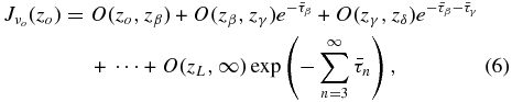
where we have denoted with the symbol O(zi, zj) the “Olbers' integrals” on the right-hand side of Equation (2), calculated between redshifts zi and zj > zi and with  equal to the relevant continuum opacity,

In Equation (6), zL = (1 + zo)(νL/νo) − 1, νL is the frequency at the Lyman limit, and  are the Lyman-series effective opacities at redshifts zβ, zγ, zδ, .... In the case of resonant absorption by H i, the LyC optical depth
  is zero in all O-integrals except the last, while in the case of He ii all terms must include photoelectric absorption by H i and He i (as well by He ii in the last term). Equation (6) is easily generalized to higher observed frequencies, νn < νo < νn + 1, to read

Note how, in the case of large resonant opacities, only sources between the observer and the “screen” redshift zn = (1 + zo)(νn/νo) − 1 corresponding to the frequency of the nearest Lyman-series line above νo will not be blocked from view: the background energy spectrum will show a series of discontinuities, peaking at frequencies just above each resonance, as the first integral in Equation (8) extends over the largest redshift path, and going to zero at resonance.
2.3. Lyman Series Cascades
Each photon absorbed through a Lyman series resonance causes a radiative cascade that ultimately terminates either in a Lyα photon or in two-photon 2s → 1s continuum decay. In the former case the photon scatters until it is redshifted out of resonance, in the latter the photons escape to infinity without further interactions. Consider, for example, the absorption of a Lyβ photon. The excited 3p level is depopulated via 3p → 2s decay (Hα). In the low-density IGM, collisional l-mixing of the 2s–2p levels (Seaton 1959) is negligible, and the cascade can only terminate in two-photon 2s → 1s emission (Hirata 2006). Without l-mixing, the quantum selection rules forbid Lyβ photons from being converted into Lyα: by contrast, excitation of the 4p level by absorption of Lyγ can decay via the 3s or 3d levels to the 2p and ultimately produce Lyα. More generally, the fraction, fn, of decays from an np state that generates Lyα photons can be determined from the selection rules and the decay probabilities. This fraction is found to increase as fn = (0, 0.2609, 0.3078, 0.3259, …) for n = (3, 4, 5, 6, …) and to asymptote to 0.359 at large n (Pritchard & Furlanetto 2006). Note that this is valid in the approximation that the IGM is optically thick to higher-order Lyman-series transitions.
What is the Lyα diffuse flux produced by these Lyman-series cascades? Let  be the background intensity measured just above the H i or He ii Lyn resonance at redshift z. The Lyn flux that is absorbed and converted into Lyα is
 ![$f_n J_{\nu _n}(z)[1-e^{-\bar{\tau }_n(z)}]$](https://content.cld.iop.org/journals/0004-637X/746/2/125/revision1/apj412591ieqn8.gif) , and the proper Lyα volume emissivity generated by this process can be written as
, and the proper Lyα volume emissivity generated by this process can be written as

where δ(x) is the Dirac delta function. The additional flux observed at frequency νo ⩽ να and redshift zo from this process is then

(Madau & Haardt 2009), where 1 + zα = (1 + zo)(να/νo) and the LyC optical depth  is zero in the case of resonant absorption by H i. When summing up over all Lyman series lines, the term in square brackets must be replaced by
 ![$\sum _{n>3}\lbrace f_n J_{\nu _n}(z_\alpha)[1-e^{-\bar{\tau }_n(z_\alpha)}]\rbrace$](https://content.cld.iop.org/journals/0004-637X/746/2/125/revision1/apj412591ieqn10.gif) . The same Lyn cascade also produces a two-photon continuum with emissivity given by
. The same Lyn cascade also produces a two-photon continuum with emissivity given by

where the two-photon emission function fν is expressed in the photons per unit frequency interval and is symmetric about να/2.
We note that the underlying assumption in Equations (9) and (11) is that every absorber is a source of unprocessed Lyα line and two-photon continuum radiation, i.e., that these photons escape into intergalactic space without appreciable local absorption. In the case of He ii Lyα emission, this requires negligible “in situ” destruction from dust, metals (O iii Bowen fluorence), and photoelectric absorption by H i, so that the Lyα photons diffuse into the wings and eventually escape from the production site into the IGM. This is a good approximation at the low metallicities that characterize intergalactic absorbers (Kallman & McCray 1980), even more so since the reprocessing of Lyman series photons occurs in a “skin” layer at the surface of an absorption system. In Section 4 we will show that this is a poor approximation in the case of the reprocessing of LyC radiation, a proper treatment of which requires a numerical solution of the radiative transfer equation within individual absorbers.
3. DISTRIBUTION OF ABSORBERS ALONG THE LINE OF SIGHT
The effective opacity of the IGM has traditionally been one of the main uncertainties affecting calculations of the UV background. Our improved model uses a piecewise power-law parameterization for the distribution of absorbers along the line of sight,

and is designed to reproduce accurately a number of recent observations.
- 1.Over the column density range
 , we use (A, β, γ) = (1.2 × 10⁷, 1.5, 3.0), where the normalization A is expressed in units of cm−2(β − 1), and β = 1.5 is chosen following, e.g., Tytler (1987). As noted, e.g., by Meiksin & Madau (1993), Petitjean et al. (1993), and Kim et al. (1997, 2002), starts to steepen from the empirical −1.5 power law at . Here, we assume (A, β, γ) = (3.8 × 10¹⁴, 2.0, 3.0) for . A “curve of growth” analysis (providing the relationship between equivalent width and column density) with Doppler parameter b = 32 km s−1, together with Equation (5) and the above distribution of Lyα-forest clouds, produces a Lyα effective opacity , in agreement with the best fits of Faucher-Giguère et al. (2008b) after metal correction.
 - 2.At the other end of the column density distribution, a recent survey of damped Lyα systems (DLAs) by Prochaska & Wolfe (2009) (see also Guimaraes et al. 2009) yields DLAs per unit redshift at 〈z〉 = 3.7 above . With a power-law exponent β = 2 down to a break column of (Prochaska & Wolfe 2009), and with an incidence per unit redshift ∝(1 + z)1.27 (Rao et al. 2006), the parameters for the DLAs become (A, β, γ) = (8.7 × 10¹⁸, 2, 1.27).
- 3.For absorbers with (the so-called super Lyman-limit systems, or SLLSs), we use O'Meara et al. (2007), who find dN/dz = 0.97 SLLSs per unit redshift at 〈z〉 = 3.5 above . Matching with the DLAs abundance then requires (A, β, γ) = (0.45, 1.05, 1.27) for the SLLSs.
- 4.There is obviously a significant mismatch between the power-law exponent for the Lyα clouds (γ = 3) and the SLLSs (γ = 1.27). Continuity then requires the shape of to change with redshift over the column density range of the Lyman-limit systems (LLSs), . In this interval of column densities we match the distribution function with a power law of redshift-dependent slope. The procedure yields the slopes β = 0.47, 0.61, 0.72, 0.82 at redshifts z = 2, 3, 4, 5, respectively, in agreement with Prochaska et al. (2010) who find for the LSSs β = 0.8+0.4−0.2 at z ≈ 3.5.
- 5.The ensuing distribution is shown in the left panel of Figure 1 for z = 2, 3.5, 5 where, for clarity, we have multiplied the values at the highest and lowest redshift by 50 and 1/50, respectively. Its shape is similar to the distribution inferred by Prochaska et al. (2010). In the right panel of the same figure we have plotted the quantity , i.e., the effective optical depth at 1 ryd per unit redshift per unit logarithmic interval of hydrogen column. This shows the dominant contribution of the LLSs and SLLSs to the LyC opacity.
- 6.The above parameterizations reproduce well the observations at 2 ≲ z ≲ 5. At low redshift, however, Hubble Space Telescope (HST) data show that the forest undergoes a much slower evolution. Following Weymann et al. (1998) we take γ = 0.16 in the interval 0 < z < zlow and dN/dz = 34.7 at z = 0 above an equivalent width of 0.24 Å (corresponding to a column of 1013.87 cm−2 for b = 32 km s−1). We derive (A, β, γ) = (1.73 × 10⁸, 1.5, 0.16) for and (A, β, γ) = (5.49 × 10¹⁵, 2, 0.16) for at all redshifts below zlow = 1.56. We use a broken power law for the redshift distribution of the SLLSs and DLAs as well; assuming that the same γ = 0.16 slope and transition redshift zlow inferred for the forest also hold in the case of the thicker absorbers, we derive a normalization at z < zlow of A = 1.28 for the SLLSs and A = 2.47 × 10¹⁹ for the DLAs. This yields dN/dz = 0.74 absorbers above at 〈z〉 = 0.69, in agreement with the value measured by Stengler-Larrea et al. (1995), dN/dz = 0.70 ± 0.2.
- 7.Above z = 5.5, the spectra of the highest redshift quasars known show an accelerated evolution in the Lyα opacity of the IGM, (Fan et al. 2006b), indicating a sharp increase in the average neutrality of the universe. This can be mimicked by assuming for the forest the values (A, β, γ) = (29.5, 1.5, 9.9) () and (A, β, γ) = (9.35 × 10⁸, 2, 9.9) () above redshift 5.5.













![$N_{{\rm H\,\mathsc{i}}}d\bar{\tau }_c/(dz dN_{{\rm H\,\mathsc{i}}})\vert _{\nu =\nu _{912}}=N_{{\rm H\,\mathsc{i}}}f(N_{{\rm H\,\mathsc{i}}},z) [1-\exp (-N_{{\rm H\,\mathsc{i}}}\sigma _{912}]$](https://content.cld.iop.org/journals/0004-637X/746/2/125/revision1/apj412591ieqn24.gif)



![$\bar{\tau }_\alpha =2.68[(1+z)/6.5]^{10.9}$](https://content.cld.iop.org/journals/0004-637X/746/2/125/revision1/apj412591ieqn28.gif)


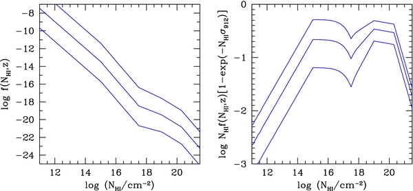
Figure 1. Left: the assumed distribution of absorbers in H i column density at redshift z = 2 (bottom curve), z = 3.5 (middle curve), and z = 5 (top curve). For clarity, we have multiplied the top and bottom curves by 50 and 1/50, respectively. Right: the quantity ![$N_{{\rm H\,\mathsc{i}}}f(N_{{\rm H\,\mathsc{i}}},z) [1-\exp (-N_{{\rm H\,\mathsc{i}}}\sigma _{912}]$](https://content.cld.iop.org/journals/0004-637X/746/2/125/revision1/apj412591ieqn35.gif) at the same redshifts, showing the dominant contribution of the optically thick LLSs and SLLSs to the intergalactic opacity at 1 ryd.
at the same redshifts, showing the dominant contribution of the optically thick LLSs and SLLSs to the intergalactic opacity at 1 ryd.
Download figure:
Standard image High-resolution imageThe parameters of the adopted distribution of intergalactic absorbers are summarized in Table 1.
Table 1. Parameters of the Distribution of Intergalactic Absorbers
| Absorbers Class | log  cm−2) cm−2) |
β | A [cm−2(β − 1)] | γ | Redshift |
|---|---|---|---|---|---|
| Lyα forest | 11–15 | 1.5 | 107.079 | 3.0 | 1.56 < z < 5.5 |
| 11–15 | 1.5 | 108.238 | 0.16 | z < 1.56 | |
| 11–15 | 1.5 | 101.470 | 9.9 | z > 5.5 | |
| 15–17.5 | 2.0 | 1014.580 | 3.0 | 1.56 < z < 5.5 | |
| 15–17.5 | 2.0 | 1015.740 | 0.16 | z < 1.56 | |
| 15–17.5 | 2.0 | 108.970 | 9.9 | z > 5.5 | |
| LLSs | 17.5–19 | ||||
| SLLSs | 19–20.3 | 1.05 | 10−0.347 | 1.27 | z > 1.56 |
| 19–20.3 | 1.05 | 100.107 | 0.16 | z < 1.56 | |
| DLAs | 20.3–21.55 | 2.0 | 1018.940 | 1.27 | z > 1.56 |
| 20.3–21.55 | 2.0 | 1019.393 | 0.16 | z < 1.56 | |
Download table as: ASCIITypeset image
3.1. Mean Free Path of Hydrogen-ionizing Radiation
Inserting our  into Equation (3), we can compute the (proper) LyC mean free path for 1 ryd photons as

This is plotted in the left panel of Figure 2 in the redshift range 3.5–4.5. At z = 3.5, the major contributors to the LyC opacity are, in order of decreasing magnitude, the high column-density Lyα forest ( , 32%), the SLLSs (28%), the LLSs (20%), the low column-density Lyα forest (
 , 12%), and the DLAs (8%). A new method to directly measure the IGM LyC opacity along quasar sight lines has been recently presented by Prochaska et al. (2009). The approach analyzes the “stacked” spectrum of 1800 quasars drawn from the Sloan Digital Sky Survey (SDSS) to give an empirical determination of the mean free path λ912mfp. Our new opacity model agrees very well with the measurements of Prochaska et al. (2009) and produces a continuum opacity that is approximately half of that adopted in Paper II. The right panel of the same figure shows how our model also provides a good fit to the Lyα quasar transmission data over the entire redshift range 2 ≲ z ≲ 6.
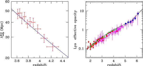
Figure 2. Left: the predicted proper mean free path at 1 ryd (solid line) together with the measurements of Prochaska et al. (2009) (crosses). Right: evolution of the observed effective Lyα optical depth,  , where
  is the transmitted flux ratio. Data points are from Schaye et al. (2003; red filled circles), Songaila (2004; magenta empty squares), Faucher-Giguère et al. (2008b; green filled squares), and Fan et al. (2006b; blue filled circles). The solid line shows the Lyα opacity,
  , predicted by Equations (5) (for n = 2) and (12), and using a curve-of-growth analysis corresponding to a Doppler parameter b = 32 km s−1.
Download figure:
Standard image High-resolution imageFor a single population of absorbers described by Equation (12), the mean free path scales with frequency and redshift as λmfp(ν, z)∝(ν/ν912)3(β − 1)H−1/(1 + z)γ + 1. Given the multi-component distribution summarized in Table 1, we can readily compute the mean free path of ionizing radiation in the range 13.6 ⩽ hν < 48.4 eV under the assumption that He i continuum absorption at energies above 24.2 eV can be neglected (photons between 48.4 and 54.4 eV are reprocessed by He ii Lyman series resonance absorption, see Section 2.2). For ease of use in analytical calculations, we fit our numerical results for the mean free path as

where s ≡ ν/ν912. Both the normalization A(s) and the exponent γ(s) are well fit by third-order polynomials of the form

Numerical values of the best-fit polynomial coefficients are given in Table 2: the fitting function is adjusted to be continuous in value at the redshifts where it changes slope. As discussed above, the fit is only valid in the range 1 ⩽ s ⩽ 3.56. Close to the hydrogen Lyman edge, and at early enough epochs, only “local” radiation sources—sources within a mean free path of a few tens of Mpc—contribute to the ionizing background intensity, and one can neglect cosmological effects such as source evolution and frequency shifts. In this “source-function” approximation, 4πJ912(z) ≈ 912(z) λ912mfp(z).
Table 2. Fitting Parameters for the Hydrogen LyC Mean Free Path
| Parameter | p3 | p2 | p1 | p0 | |
|---|---|---|---|---|---|
| A | 0.0509 | −0.406 | 1.167 | 1.076 | |
| 0 < z < 1.56 | γ | 0. | 0. | 0. | −0.160 |
| 1.56 < z < 5.5 | γ | 0.0593 | −0.519 | 1.586 | −2.104 |
| z > 5.5 | γ | 0.122 | −1.356 | 5.998 | −8.423 |
Download table as: ASCIITypeset image
4. PHOTOIONIZATION STRUCTURE OF ABSORPTION SYSTEMS
The ionization state of individual absorbers enters in calculations of the He i and He ii opacities and of the continuum and line recombination radiation from hydrogen and helium. Under the assumption of photoionization equilibrium (generally accurate for quasar absorbers, see Paper II), in a pure H/He gas illuminated by a local radiation intensity  , the ion fractions
  ,
,  , and
, and  can be written in implicit form as

where

Γi is the photoionization rate of species i ∈ {H i, He i, He ii},

and αi is the (case A) recombination coefficient to all atomic levels of species i. The recombination rate of the next ionization state i + 1 (e.g., if i is H i then i + 1 is H ii) is neni + 1αi, where the electron number density ne is

In the case of a highly ionized medium with  ,
,  ,
,  , the densities of He i and He ii can be expressed in terms of the H i density as

and

For optically thin systems, the above relations with  clearly give the ratio between the column densities of different ions. Note how the quantity

is independent on gas density only as long as the optically thin approximation holds, while the ratio

is always density dependent.
4.1. Slab Approximation and Fitting Formulae
An iterative solution to the equations of cosmological radiative transfer that included a detailed numerical calculation of the ionization and temperature structure of individual absorbers at every timestep would be a very computing-intensive task. To properly treat the self-shielding of LyC radiation, in Paper II we modeled absorbers as semi-infinite slabs, developed a “steplike” approximation to the function  , and used an analytical escape probability formalism to include the recombination emission from absorbers. Fardal et al. (1998) solved the local radiative transfer problem via an integral equation (the Milne solution for a gray atmosphere) for the number of photoionizations at any optical depth in a given slab. They also devised an approximation formula to η that closely followed the numerical results. Faucher-Giguère et al. (2009) have recently generalized the treatment of Fardal et al. (1998) and applied a similar fitting formula to the results of a code that self-consistently solves the photoionization equilibrium balance, including the influence of recombination radiation. Here, we follow a similar method: under the assumption of Jeans length thickness for the absorbers, we solve the ionization and thermal structure of a slab of finite width illuminated by an external isotropic radiation field Jν, and derive analytical approximations for the ratios η and ζ as a function of
  . Details of our calculations are provided in the Appendix. We parameterize the external background flux as a power law, Jν = J912(ν/ν912)−α, and as in Faucher-Giguère et al. (2009) divide the intensity above 54.4 eV by a factor of 10 to mimic a cosmological UV filtered spectrum.
Figure 3 shows the resulting ratios  and
and  for a range of input spectra and for the representative intensity value at 1 ryd of 10−22 erg cm−2 s−1 Hz−1 sr−1. The function η remains constant at low H i columns, as long as the optically thin approximation holds. As the neutral hydrogen column increases, the slab first becomes optically thick to He ii-ionizing radiation and η increases. Slabs with even larger columns become optically thick to H i LyC: they are characterized by a highly ionized surface layer and an almost fully neutral core. This is the reason for the rapid decrease of η after the peak and the consequent trend of ζ toward the neutral limit, ζ → nHe/nH. As in Fardal et al. (1998) and Faucher-Giguère et al. (2009), we calculate the column
  from the equation

where  ,
,  , and A and B are constants fitted to our numerical results. To make use of the above expression, one must further specify the ionization rates Γi to be used in the Ri terms together with a relation between electron density and
  . It is in this second step that our approach differs from that of Faucher-Giguère et al. (2009). These authors used the optically thin limit for Γi, which provides a poor approximation to the numerical results. Here, we first compute the ionization rates in the optically thin limit,

and derive ηthin using Equation (21). For a given (input value) of  , we then calculate
  . We then write a first-order approximation to the He ii ionization rate at the face of the slab,

The analogous expression for H i is

Finally, we compute the Ri factors for H i and He ii in Equation (24) as

The recombination rates depend on the gas temperature. We found that our numerical results can be fit with the simple scaling

where J912, −22 ≡ J912/10−22 erg cm−2 s−1 Hz−1 sr−1 is adequate for our purposes. The weak dependence on J is related to the fact that, for  , cooling is largely provided by collisionally excited line radiation rather than by recombinations. With this simplified treatment, we have been able to fit the numerically obtained values of η for a broad range of input spectra. The best-fit curves shown in the left panel of Figure 3 have been obtained taking A = 0.02 and B = 0.25 in Equation (24), and

for the electron density. Here,  and
and  . The above relation can be derived assuming Jeans length thickness for the absorbers and optically thin photoionization equilibrium (Schaye 2001; see also Faucher-Giguère et al. 2009). A simple approximation for ζ can also be derived, once η is obtained. We use Equation (20),
  , with
  for
for  cm−2. At larger columns we apply a linear (in log space) extrapolation to the limiting vale ζ → nHe/nH assumed to be reached at
  cm−2.
cm−2.
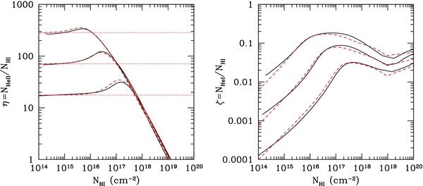
Figure 3. Left panel: the ratio  as a function of
  at redshift 3. The illuminating spectrum has intensity Jν = J912(ν/ν912)−α, with J912, −22 = 1 and, from bottom to top, spectral slopes α = 0, 1, 2, with a break of a factor of 10 at 54.4 eV. Solid curves: full numerical photoionization calculations. Dashed curves: our analytical approximations for η based on Equation (24). Dotted curves: optically thin limit. Right panel: same for
  .
.
Download figure:
Standard image High-resolution image5. RECOMBINATION EMISSIVITY
In Section 2, we have seen how background photons absorbed through a Lyman series resonance cause a radiative cascade that ultimately terminates either in a Lyα photon or in two-photon 2s → 1s continuum decay. In this section, we use the detailed photoionization structure of absorbing systems to calculate the reprocessing of background LyC radiation by the clumpy IGM via atomic recombination processes. We include recombinations from the continuum to the ground state of H i, He i, and He ii, as well as He ii Balmer, two-photon, and Lyα emission. Using the formalism developed in the Appendix, the recombination flux at the slab surface,

can be written as
The emission coefficient from a generic recombination process,

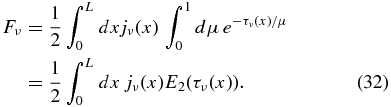
where ϕν is the normalized emission profile and αr is the relevant recombination coefficient, is proportional to the density of species i, times the rate at which it absorbs ionizing photons (Γi), times the fraction of recombinations that lead to the radiative transition under consideration (the ratio αr/αi). The emission profile of free-bound recombination radiation can be computed via the Milne detailed-balance relation, which relates the velocity-dependent recombination cross section to the photoionization cross section, while a delta-function profile is sufficient for bound–bound transitions. The cosmological proper recombination emissivity for the relevant recombination process can then be computed by integrating over the distribution of absorbers,

where the factor two accounts for the two surfaces of a slab. Using Equations (32) and (33), and denoting with Ni = ∫L0nidx the species i column density of the absorber, the recombination emissivity becomes
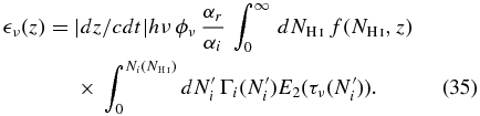
As with the ionization and thermal structure of individual absorbers, it is not practical to perform a self-consistent, iterative, numerical evaluation of the recombination emissivity at every timestep in the cosmological code. To derive a simple analytical formula to the emergent radiation from absorbers, we make use of the fact that the number of ionizing incident photons that are absorbed saturates in the optically thick regime, and approximate the second integral on the right-hand side of Equation (35) as (see Faucher-Giguère et al. 2009)

Here NT is the column density of ion i above which the recombination emission saturates. As shown in Figure 4, the above formula works especially well in the case of LyC recombination re-emission from H i and He ii, where self-absorption by the emitting ion dominates the local reprocessing of recombination radiation. Our best-fit parameters to the full numerical results for H i, He i, and He ii LyC recombinations are NT = 6.5 × 10¹⁶ (ν/ν912)1.5 cm−2, NT = 1.2 × 10¹⁶ (ν/ν504)1.5 cm−2, and NT = 2.3 × 10¹⁷ (ν/ν228)1.5 cm−2, respectively. (In the case of non-ionizing H i recombination Lyα and two-photon emission, we find NT = 6.5 × 1017 cm−2.)
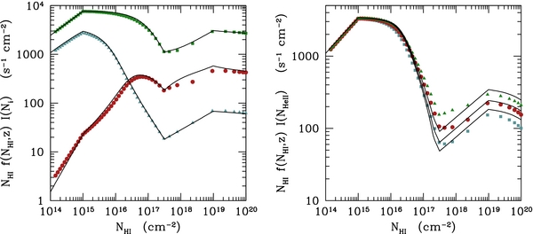
Figure 4. Left panel: LyC recombination radiation from quasar absorbers as a function of  . The points depict the results of the full numerical integration of the local radiative transfer equation, while the lines show our analytical approximations (Equation (36)). Green squares: H i LyC at 912 Å. Blue triangles: He ii LyC at 228 Å. Red circles: He i LyC at 504 Å. The quantity plotted is the integral I(Ni) (Equation (36)) multiplied by
  (Equation (12)) at z = 3, showing the contribution of optically thin and optically thick absorbers to the LyC emissivity. For this comparison we assumed an illuminating spectrum with J912, −22 = 1 and spectral slope α = 1, with a break of a factor of 10 at 54.4 eV. Right panel: same as left panel, but for recombination re-emission from He ii BalC at 13.6 eV (blue squares), Lyα at 40.8 eV (green triangles), and two-photon continuum at 20.4 eV (red circles).
Download figure:
Standard image High-resolution imageThe emergent recombination flux from He ii BalC, two-photon, and Lyα depends on the helium (emission) as well as hydrogen (absorption) ionization structure. With the adopted column density distribution, however, recombinations into He ii are dominated by absorbers in the range of columns  cm −2: in these systems, H i absorption can be neglected and a simple approximation can be found by setting NT = 2.3 × 1018 cm−2. The fit at large H i columns is actually improved by multiplying the right-hand side of Equation (36) by exp [ − min(τ912, 1.3)](ν912/ν)0.6. A comparison between the results of the full numerical integration of the local radiative transfer equation and our analytical approximations to the recombination radiation from He ii BalC, two-photon, and Lyα are shown in the right panel of Figure 4. Note that, in our calculations, we have again assumed that He ii Lyα photons diffuse into the wings and then escape subject only to continuum absorption.
6. QUASAR UV EMISSIVITY
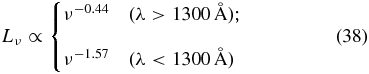
The only sources of ionizing radiation included in CUBA are star-forming galaxies and quasars. For the quasar comoving emissivity at 1 ryd, 912(z)/(1 + z)3, we use the function
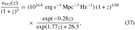
which closely fits the results of Hopkins et al. (2007) in the redshift interval 1 < z < 5. The UV SED is given by the broken power law
7. QUASAR X-RAY EMISSIVITY
The extrapolation of the steep UV power law in Equation (38) to higher energies is unable to reproduce the X-ray properties of the quasar population as a whole, as recorded in the cosmic XRB. The XRB may play a unique role in regulating the thermodynamics and ionization degree of intergalactic absorbers. In a photoionized IGM, soft X-rays between 0.5 and 0.9 keV are responsible for the highest ionization states of metals like carbon, nitrogen, and oxygen. At early epochs, X-rays penetrate regions that are optically thick to UV radiation, providing a source of heating and ionization. They could make the IGM warm and weakly ionized prior to the era of reionization breakthrough (e.g., Oh 2001; Venkatesan et al. 2001; Madau et al. 2004; Ricotti & Ostriker 2004; Kuhlen & Madau 2005). Compton scattering of hard XRB photons may be a source of heating for highly ionized low-density intergalactic gas (Madau & Efstathiou 1999).
Deep X-ray surveys aided by optical identification programs have shown that the bulk of the XRB is produced by a mixture of unobscured “Type 1” and obscured “Type 2” AGNs (Mushotzky et al. 2000; Giacconi et al. 2001), as predicted by XRB synthesis models constructed within the framework of AGN unification schemes (e.g., Setti & Woltjer 1989; Madau et al. 1994; Comastri et al. 1995; Gilli et al. 2007). Here, we compute the total X-ray emissivity from Type 1 and Type 2 AGNs following a modern version of the original approach by Madau et al. (1994).
7.1. Intrinsic Hard X-ray Luminosity Function
According to Ueda et al. (2003), who combined various surveys from the HEAO-1, ASCA, and Chandra satellites, the hard 2–10 keV quasar luminosity function (HXLF) follows a luminosity-dependent density evolution with a cutoff redshift (above which the evolution stops) that increases with luminosity. At the present epoch, the intrinsic (i.e., before absorption) HXLF of all AGNs (including both Type 1's and Type 2's) is best represented by

in the luminosity range 1041.5–1046.5 erg s−1, where ϕ* = 2190 Gpc−3 and L* = 1043.94 erg s−1. This changes with cosmic time (for redshift up to 3) as

where the evolution factor is
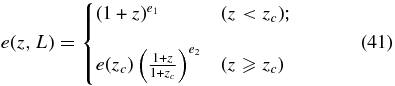
and

Here, e1 = 4.23, e2 = −1.5, z*c = 1.9, and La = 1044.6 erg s−1 (Ueda et al. 2003). An extension of the HXLF up to z ∼ 5 by Silverman et al. (2008) shows a steeper decline in the number of z > 3 AGNs with an evolution rate similar to that found by studies of optically selected QSOs. The new fit requires a much stronger evolution above the cutoff redshift, e2 = −3.27, than previously found by Ueda et al. (2003, e2 = −1.5). In the following, we shall use Ueda et al.'s (2003) HXLF best-fit parameters together with the Silverman et al. (2008) value for e2.
For the intrinsic spectrum before absorption, we assume the standard power law multiplied by an exponential,

with α = 0.9 (Nandra & Pounds 1994). The high-energy cutoff, Ec = 460 keV, is fixed by the shape of the XRB turnover above 30 keV. These seed photons are then reflected toward the observer by a semi-infinite cold disk close to the primary emitter. This reflection component, commonly detected in the X-ray spectra of nearby Seyfert galaxies (Nandra & Pounds 1994), is comparable to the direct flux around 30 keV, decreases rapidly toward lower energies, and flattens the overall spectral slope above 10 keV (Lightman & White 1988).
7.2. AGN Emissivity After Absorption
According to the AGN unification scheme, obscuring matter at a distance of several parsecs from the central powerhouse blocks our line of sight to the active nucleus. When our view is unobscured, we see a Type 1 AGN; when our view is occulted, photons of all energies from the far IR to several keV are absorbed, and in these bands we can only detect the nucleus in scattered light. Ueda et al. (2003) found the following expression for the observed (normalized) distribution of absorbing NH columns:

where the parameter

accounts for the fact that the fraction of absorbed sources is smaller at higher luminosities. Here, ψmax = (1 + )/(3 +
),
= 1.7, ψ44 = 0.47, β = 0.1, and ∫2420f(L, NH) dlog NH = 1. Sources absorbed by a column larger (smaller) than 1022 cm−2 are defined as X-ray Type 2 (Type 1) AGNs. It is assumed that “Compton-thick” AGNs with columns log NH > 24 are not present in samples detected below 10 keV. Such a population is added by extrapolating the NH function above log NH > 24, keeping the same normalization up to log NH = 25 as well as the same cosmological evolution of Compton-thin AGNs (Ueda et al. 2003).
We then follow Madau et al. (1993) and model the thick blocking material that covers most of the solid angle around the central X-ray source as a homogeneous spherical cloud of cold material and column NH. The radiation transfer is computed with a Monte Carlo code constructed using the photon-escape weighing method of Pozdnyakov et al. (1983). We set the electron temperature equal to zero, use the full Klein–Nishina scattering cross section, adopt the bound-free opacity associated with standard cosmic-abundance material from Morrison & McCammon (1983), and ignore the iron Kα emission line in the spectra. Each Monte Carlo run uses 106 photons and produces as output an absorbed spectrum, SE(NH). After being reprocessed by cold material along the line of sight, the emergent specific intensity forms a hump, whose position and width are determined by the competition of bound-free absorption at low energies, and Compton downscattering and exponential roll-off of the primary spectrum at high energies (Madau et al. 1993). A small spectral component, equal to 2.5% of the primary incident power and representing the flux scattered into the line of sight by electrons in the warm ionized medium, is added to the transmitted Type 2 flux. The absorbed spectra are then averaged over the NH-distribution corresponding to a given luminosity, and normalized to the unabsorbed 2–10 keV flux,

to yield a flux normalized, luminosity-dependent, average AGN SED. The X-ray proper emissivity as a function of redshift is then obtained by simply integrating over the HXLF,

where we set Lmin = 1041.5 erg s−1 and Lmax = 1048 erg s−1.
The model described above is able to reproduce a number of X-ray observations, from the evolution of AGNs in the soft and hard X-ray bands, to the XRB. The quasar comoving emissivity at 2 keV and 10 keV is plotted in Figure 5, while a global fit to the XRB is shown in the left panel of Figure 6. The absolute XRB flux is still affected by rather large uncertainties: our model reproduces well the background intensity measured by HEAO-1 and BeppoSAX, but the HEAO-1 A2 data are lower by about 20% with respect to the determinations by, e.g., XMM and RXTE at energies below 10 keV. Figure 6 (right panel) depicts the broadband quasar comoving emissivity per logarithmic bandwidth, νν/(1 + z)3, as a function of photon energy from the optical to hard X-rays. In terms of energy output, the composite spectrum for λ < 5000 Å is characterized by two broad bumps, one in the UV at 10 eV and another in the X-ray region at 30 keV (a third peak in the mid-infrared, see, e.g., Sazonov et al. 2004, can be neglected for the present purposes). While X-rays dominate the energy output at z = 0, the peak of the emitted power moves increasingly toward the UV at redshifts above 1.
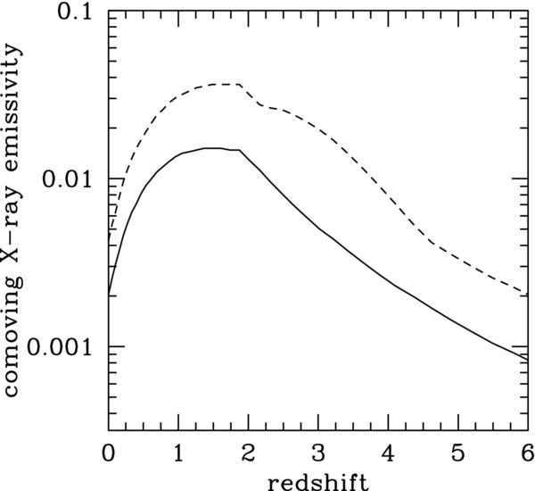
Figure 5. Quasar comoving emissivity at 2 keV (dashed line) and 10 keV (solid line) in units of 1023 erg s−1 Mpc−3 Hz−1. The latter has been computed following Ueda et al. (2003) and Silverman et al. (2008), the former using the procedure outlined in Section 7.2.
Download figure:
Standard image High-resolution image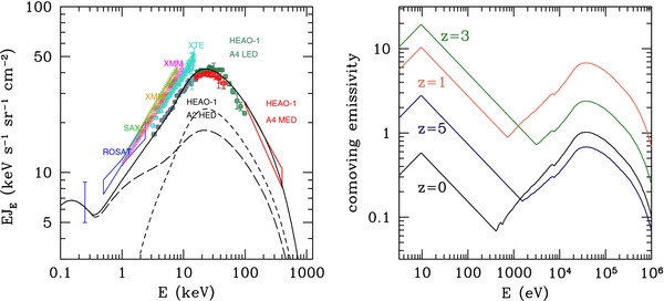
Figure 6. Left panel: the cosmic XRB spectrum and the predicted contribution from AGNs. Gray points: HEAO-1 A2 HED data (Gruber et al. 1999). Dark green points: HEAO-1 A4 LED (Gruber et al. 1999). Cyan points: Rossi-XTE (Revnivtsev et al. 2003). Blue point: 0.25 keV soft XRB intensity from ROSAT shadowing experiments (Warwick & Roberts 1998). Red bowtie: HEAO-1 A4 MED (Kinzer et al. 1997). Blue bowtie: ROSAT PSPC data (Georgantopoulos et al. 1996). Light green bowtie: BeppoSAX (Vecchi et al. 1999). Purple and yellow bowties: Newton-XMM (Lumb et al. 2002; De Luca & Molendi 2004). Solid line: our synthesis model spectrum, produced by a mixture of absorbed (log NH > 22, short-dashed line) and unabsorbed (log NH < 22, long-dashed line) AGNs. See the text for details. Right panel: the broadband quasar comoving emissivity per logarithmic bandwidth, νν/(1 + z)3 (in units of 1039 erg s−1 Mpc−3), as a function of photon energy E from the optical to hard X-rays. The composite spectrum is shown at redshifts z = 0, 1, 3, 5.
Download figure:
Standard image High-resolution image8. GALAXY EMISSIVITY
Star-forming galaxies are expected to play a dominant role as sources of hydrogen-ionizing radiation at z > 3 as the quasar population declines with look-back time. To compute the LyC emissivity from galaxies at all epochs, we start with an empirical determination of the star formation history of the universe following Madau et al. (1996). We adopt the far-UV (FUV, 1500 Å) luminosity functions of Schiminovich et al. (2005) in the redshift range 0 ⩽ z ⩽ 2, of Reddy & Steidel (2009) at z = 2.3 and 3.05, and of Bouwens et al. (2011) at redshifts 3.8, 5.0, 5.9, 6.8, and 8.0. All were integrated down to Lmin = 0.01 L* using Schechter function fits with parameters (ϕ*, L*, α) to compute the dust-reddened galaxy FUV luminosity density ρFUV,3

Here α denotes the faint-end slope of the Schechter parameterization and Γ is the incomplete gamma function. We used α = −1.6 at 0 < z < 2, α = −1.73 at z = 2.3 and z = 3.05, and α = −1.73, −1.66, −1.74, −2.01, −1.91 at z = 3.8, 5.0, 5.9, 6.8, 8.0, respectively (see Schiminovich et al. 2005; Reddy & Steidel 2009; Bouwens et al. 2011).
Dust attenuation was treated using a Calzetti et al. (2000) extinction law, with the function

measuring the magnitudes of attenuation suffered at frequency ν and redshift z. For the luminosity-weighted obscuration at 1500 Å we take

The above expression reproduces at z ⩽ 2 the FUV “minimum dust correction factor” of 2.5 from Schiminovich et al. (2005), the dust correction factors of 2.38 ± 0.59 and 2.0 ± 0.62 at z = 2.3 and z = 3.05 from Reddy & Steidel (2009), and the decreasing dust attenuation at higher redshift from Bouwens et al. (2011). The dust-corrected luminosity densities were smoothed with an approximating function and then compared with the results of spectral population synthesis models as follows. The GALAXEV library of Bruzual & Charlot (2003) provides the age–luminosity evolution for a simple stellar population (SSP) at different wavelengths. The FUV luminosity density (before dust obscuration) at time t of a “cosmic stellar population” characterized by a star formation rate density SFRD(t) and a metal-enrichment law Z(t) is given by the convolution integral

where lFUV[τ, Z(t − τ)] is specific luminosity radiated at 1500 Å per unit initial stellar mass by an SSP at age τ and metallicity Z(t − τ). We use SSPs of decreasing metallicities with redshift according to

(Kewley & Kobulnicky 2007), for a Salpeter IMF between 0.1 and 100 M☉. Starting from an initial guess, the function SFRD(t) was adjusted in an iterative fashion until the computed FUV luminosity densities as a function of redshift provided a good match to the data. The best-fitting star formation history,

is shown in Figure 7 (left panel), together with the observed luminosity densities adopted in this study. The latter have been converted to ongoing star formation rate densities according to

where ρFUV is expressed in units of erg s−1 Mpc−3 Hz−1 and SFRD is in units of M☉ yr−1 Mpc−3. This approximate transformation makes use of the basic property that the FUV continuum in galaxies is dominated by short-lived massive stars and is therefore a direct measure, for a given IMF and dust content, of the instantaneous star formation rate. The conversion factor  in the equation above reproduces to within 2% the results of the synthesis models above redshift 2 given the adopted star formation and metal enrichment history (see Madau et al. 1998). At redshift 0 < z < 1,
  decreases from 1.16 × 10⁻²⁸ to 1.10 × 10⁻²⁸. Note that these newly derived conversion factors are between 21% and 33% smaller than the widely used value,
  , quoted by Kennicutt (1998) (and based on the calibration by Madau et al. 1998), the differences reflecting updated stellar population synthesis models and subsolar metallicities at high redshifts.
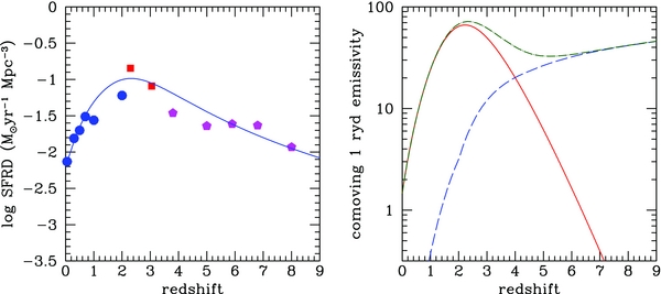
Figure 7. Left: the cosmic history of star formation. The FUV data points from Schiminovich et al. (2005) (blue dots), Reddy & Steidel (2009) (red squares), and Bouwens et al. (2011) (magenta pentagons) have been converted to instantaneous star formation rate density using the conversion factor  (see the text for details). The best-fitting star formation history, SFRD(z) = [6.9 × 10⁻³ + 0.14(z/2.2)1.5]/[1 + (z/2.7)4.1] M☉ yr−1 Mpc−3, is plotted with the solid blue curve. Right: comoving galaxy emissivity (in units of 1023 erg s−1 Mpc−3 Hz−1) of 1 ryd photons escaping into the IGM (dashed line), for an escape fraction 〈fesc〉 = 1.8 × 10⁻⁴(1 + z)3.4. The solid line shows the best-fit QSO emissivity of Equation (37) for comparison, while the dot-dashed line shows the total quasars + galaxies emissivity.
Download figure:
Standard image High-resolution imageOnce the star formation history has been determined, we use stellar synthesis models to compute the dust-reddened frequency-dependent UV emissivity as

We take C(t) ≡ 10−0.4A(ν, t) at all photon energies below 1 ryd and C(t) ≡ 〈fesc〉 above the Lyman limit. In our treatment, the escape fraction 〈fesc〉 is a free parameter that incorporates local continuum absorption by hydrogen, helium, and dust. It is the angle-averaged, absorption cross section-weighted, and luminosity-weighted fraction of ionizing radiation that leaks into the IGM from star-forming galaxies: the escaping radiation is produced not by sources in a semiopaque medium but by a small fraction of essentially unobscured sources (e.g., Gnedin et al. 2008). In the “minimal reionization model” discussed in detail in the next section, the escape fraction of photons between 1 and 4 ryd is assumed to be a steeply rising function of redshift (see also Inoue et al. 2006),

and is zero above 4 ryd. The expression above yields an escape fraction at z = 3.3 of 2.6%, comparable to the recent upper limit for L > L* Lyman break galaxies of Boutsia et al. (2011). The relatively low values of 〈fesc〉 implied by the above expression in the redshift interval from z = 2 (0.8%) to z = 5 (8%) are dictated in our model by the need to reproduce the hydrogen-ionization rates inferred from flux decrement measurements (see Figure 8 below). In the same redshift range, the escape fraction of ionizing radiation from star-forming galaxies hosting a γ-ray burst is measured to be 〈fesc〉 ⩽ 7.5% (95% c.l.) (Chen et al. 2007), in agreement with our expression. The high values predicted by Equation (56) above redshift 7, in excess of 20%, are needed to compensate for the decline in the star formation rate density and to reionize the IGM at early enough epochs. The resulting galaxy emissivity of 1 ryd photons escaping into the IGM is shown in the right panel of Figure 7. Galaxies dominate over QSOs at all redshifts z > 4 and make a negligible contribution to the ionizing background at z < 3. The total comoving emissivity from quasars + galaxies decreases only weakly from z = 3 to z = 5 and is fairly flat afterward. This trend is consistent with the conclusions reached by Bolton & Haehnelt (2007) and Faucher-Giguère et al. (2008a) from empirical measurements of the Lyα forest opacity.
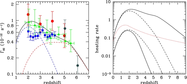
Figure 8. Left: the hydrogen photoionization rate,  , from z = 1 to z = 7. Solid curve: quasars + galaxies model. The dashed curves depict the individual contributions of the QSO population (blue) that dominates at low redshift and of the galaxy population (red) that reionize the IGM at early times. Circles: empirical measurements from the Lyα forest effective opacity by Bolton & Haehnelt (2007). Triangles: same by Becker et al. (2007) (their lognormal model). Squares: same by Faucher-Giguère et al. (2008a). Pentagons: same using the quasar proximity effect by Calverley et al. (2011). Right: the hydrogen photoheating rate per ion,
  (upper set of curves), and the He ii photoheating rate,
  (lower set of curves), from the present epoch to z = 9. All photoheating rates are expressed in units of 10−12 eV s−1. Solid lines: quasars + galaxies. Dashed lines: quasar-only. The addition of a galaxy component boosts the H i rate and decreases the He ii rate. The dotted line shows the Compton heating rate per electron in units of 10−18 eV s−1.
Download figure:
Standard image High-resolution image8.1. Lyα Emission from Galaxies
Stellar population synthesis codes do not typically include nebular line emission. Here, we provide a simple estimate of the Lyα emission from hydrogen recombinations in the interstellar medium of galaxies. In case B recombination, about 68% of all the absorbed LyC photons will be converted locally into Lyα (Osterbrock 1989). The Lyα proper volume emissivity can then be written as

where

and ν is the proper volume emissivity from galaxies. We assume here that Lyα suffers the same dust extinction as LyC, a simple treatment that is unlikely to capture the complex radiative transfer physics of the Lyα line as it propagates through the dusty ISM (see, e.g., Caplan & Deharveng 1986; Neufeld 1991; Dijkstra 2009; Scarlata et al. 2009; Dayal et al. 2010). Inserting Equation (57) into (2) yields the additional flux observed at νo ⩽ να from galaxy Lyα:

where 1 + zα = (να/νo)(1 + zo). We have neglected collisionally excited Lyα emission, as this is only about 10%–20% of the recombination term (Dayal et al. 2010). A similar contribution is also expected in the emitted spectrum of dense absorbers like the SLLSs and DLAs, while collisional excitation is always negligible in lower column density systems.
9. BASIC RESULTS
This section gives a quick overview of the main results generated by the upgraded CUBA radiative transfer code, using the formalism and parameters described above. CUBA solves the radiative transfer Equation (2) by iteration, as its right-hand term implicitly contains J in the recombination emissivity and in the effective helium opacity.
9.1. Photoionization and Photoheating Rates
The total optically thin photoionization rate of hydrogen,  , is shown in Figure 8 as a function of redshift (left panel). For comparison, we have also plotted the individual contributions of the QSO population that dominates at low redshift and of the galaxy population that reionize the IGM at early times, together with the empirical measurements from the Lyα forest effective opacity by Bolton & Haehnelt (2007), Becker et al. (2007), and Faucher-Giguère et al. (2008a), and from the quasar proximity effect by Calverley et al. (2011). The fractional recombination contribution to
  increases from 9% at z = 0 to 18% at z = 4 to up to 37% at z ≳ 7: it does so because the mean free path of recombination photons decreases with look-back time and a smaller fraction of such photons gets redshifted below the ionization threshold before capture (Faucher-Giguère et al. 2009). While the total H i photoionization rate provides a good match to the data, we note that there are large systematic uncertainties in the measurements as these depend on the assumed IGM temperature and gas density distribution.
The right panel of the same figure depicts the optically thin photoheating rates per ion (see Equation (A7) with  for the definition) of hydrogen,
  , and He ii,
  , for the quasars + galaxies and quasar-only models. The addition of a galaxy component boosts the H i rate as it increases the emissivity of hydrogen-ionizing photons at fixed H i opacity (the latter being determined by the observations). The opposite is true for He ii photoheating (as well as He ii photoionization), as galaxies do not contribute to the emissivity above 4 ryd: this increases the predicted He ii opacity (again at fixed H i opacity) and causes a large break in the background spectrum at 4 ryd and a smaller photoheating rate. While the Compton heating rate per electron is many orders of magnitude (about 7 dex at redshift 3) below the H i photoheating rate (note the different normalization of the heating rates plotted in Figure 8), it is a non-negligible source of heating for very underdense, highly ionized regions: the Compton heating rate for intergalactic gas at overdensity 0.1, temperature T = 104 K, and redshifts z = (1, 2, 3) is (53, 16, 4)% of the total photoheating rate. Table 3 tabulates the optically thin photoionization and photoheating rates of hydrogen and helium predicted by our “quasars + galaxies” model for use, e.g., in cosmological hydrodynamics simulations of the Lyα forest.
Table 3. The Cosmic Background Photoionization and Photoheating Rates
| z |  |
 |
 |
 |
 |
 |
|---|---|---|---|---|---|---|
| (s−1) | (eV s−1) | (s−1) | (eV s−1) | (s−1) | (eV s−1) | |
| 0.00 | 0.228E-13 | 0.889E-13 | 0.124E-13 | 0.112E-12 | 0.555E-15 | 0.114E-13 |
| 0.05 | 0.284E-13 | 0.111E-12 | 0.157E-13 | 0.140E-12 | 0.676E-15 | 0.138E-13 |
| 0.10 | 0.354E-13 | 0.139E-12 | 0.196E-13 | 0.174E-12 | 0.823E-15 | 0.168E-13 |
| 0.16 | 0.440E-13 | 0.173E-12 | 0.246E-13 | 0.216E-12 | 0.100E-14 | 0.203E-13 |
| 0.21 | 0.546E-13 | 0.215E-12 | 0.307E-13 | 0.267E-12 | 0.122E-14 | 0.245E-13 |
| 0.27 | 0.674E-13 | 0.266E-12 | 0.383E-13 | 0.331E-12 | 0.148E-14 | 0.296E-13 |
| 0.33 | 0.831E-13 | 0.329E-12 | 0.475E-13 | 0.408E-12 | 0.180E-14 | 0.357E-13 |
| 0.40 | 0.102E-12 | 0.405E-12 | 0.587E-13 | 0.502E-12 | 0.218E-14 | 0.429E-13 |
| 0.47 | 0.125E-12 | 0.496E-12 | 0.722E-13 | 0.615E-12 | 0.263E-14 | 0.514E-13 |
| 0.54 | 0.152E-12 | 0.605E-12 | 0.884E-13 | 0.751E-12 | 0.317E-14 | 0.615E-13 |
| 0.62 | 0.185E-12 | 0.734E-12 | 0.108E-12 | 0.911E-12 | 0.380E-14 | 0.732E-13 |
| 0.69 | 0.223E-12 | 0.885E-12 | 0.130E-12 | 0.110E-11 | 0.454E-14 | 0.867E-13 |
| 0.78 | 0.267E-12 | 0.106E-11 | 0.157E-12 | 0.132E-11 | 0.538E-14 | 0.102E-12 |
| 0.87 | 0.318E-12 | 0.126E-11 | 0.187E-12 | 0.157E-11 | 0.633E-14 | 0.119E-12 |
| 0.96 | 0.376E-12 | 0.149E-11 | 0.222E-12 | 0.186E-11 | 0.738E-14 | 0.139E-12 |
| 1.05 | 0.440E-12 | 0.175E-11 | 0.261E-12 | 0.217E-11 | 0.852E-14 | 0.159E-12 |
| 1.15 | 0.510E-12 | 0.203E-11 | 0.302E-12 | 0.251E-11 | 0.970E-14 | 0.181E-12 |
| 1.26 | 0.585E-12 | 0.232E-11 | 0.346E-12 | 0.287E-11 | 0.109E-13 | 0.202E-12 |
| 1.37 | 0.660E-12 | 0.262E-11 | 0.391E-12 | 0.323E-11 | 0.119E-13 | 0.221E-12 |
| 1.49 | 0.732E-12 | 0.290E-11 | 0.434E-12 | 0.357E-11 | 0.127E-13 | 0.237E-12 |
| 1.61 | 0.799E-12 | 0.317E-11 | 0.474E-12 | 0.387E-11 | 0.132E-13 | 0.247E-12 |
| 1.74 | 0.859E-12 | 0.341E-11 | 0.509E-12 | 0.413E-11 | 0.134E-13 | 0.253E-12 |
| 1.87 | 0.909E-12 | 0.360E-11 | 0.538E-12 | 0.432E-11 | 0.133E-13 | 0.252E-12 |
| 2.01 | 0.944E-12 | 0.374E-11 | 0.557E-12 | 0.444E-11 | 0.128E-13 | 0.244E-12 |
| 2.16 | 0.963E-12 | 0.381E-11 | 0.567E-12 | 0.446E-11 | 0.119E-13 | 0.229E-12 |
| 2.32 | 0.965E-12 | 0.382E-11 | 0.566E-12 | 0.438E-11 | 0.106E-13 | 0.207E-12 |
| 2.48 | 0.950E-12 | 0.375E-11 | 0.555E-12 | 0.422E-11 | 0.904E-14 | 0.178E-12 |
| 2.65 | 0.919E-12 | 0.363E-11 | 0.535E-12 | 0.398E-11 | 0.722E-14 | 0.145E-12 |
| 2.83 | 0.875E-12 | 0.346E-11 | 0.508E-12 | 0.368E-11 | 0.530E-14 | 0.111E-12 |
| 3.02 | 0.822E-12 | 0.325E-11 | 0.476E-12 | 0.336E-11 | 0.351E-14 | 0.775E-13 |
| 3.21 | 0.765E-12 | 0.302E-11 | 0.441E-12 | 0.304E-11 | 0.208E-14 | 0.497E-13 |
| 3.42 | 0.705E-12 | 0.279E-11 | 0.406E-12 | 0.274E-11 | 0.114E-14 | 0.296E-13 |
| 3.64 | 0.647E-12 | 0.257E-11 | 0.372E-12 | 0.249E-11 | 0.591E-15 | 0.168E-13 |
| 3.87 | 0.594E-12 | 0.236E-11 | 0.341E-12 | 0.227E-11 | 0.302E-15 | 0.925E-14 |
| 4.11 | 0.546E-12 | 0.218E-11 | 0.314E-12 | 0.209E-11 | 0.152E-15 | 0.501E-14 |
| 4.36 | 0.504E-12 | 0.202E-11 | 0.291E-12 | 0.194E-11 | 0.760E-16 | 0.267E-14 |
| 4.62 | 0.469E-12 | 0.189E-11 | 0.271E-12 | 0.181E-11 | 0.375E-16 | 0.141E-14 |
| 4.89 | 0.441E-12 | 0.178E-11 | 0.253E-12 | 0.170E-11 | 0.182E-16 | 0.727E-15 |
| 5.18 | 0.412E-12 | 0.167E-11 | 0.237E-12 | 0.160E-11 | 0.857E-17 | 0.365E-15 |
| 5.49 | 0.360E-12 | 0.148E-11 | 0.214E-12 | 0.146E-11 | 0.323E-17 | 0.156E-15 |
| 5.81 | 0.293E-12 | 0.123E-11 | 0.184E-12 | 0.130E-11 | 0.117E-17 | 0.624E-16 |
| 6.14 | 0.230E-12 | 0.989E-12 | 0.154E-12 | 0.112E-11 | 0.442E-18 | 0.269E-16 |
| 6.49 | 0.175E-12 | 0.771E-12 | 0.125E-12 | 0.952E-12 | 0.173E-18 | 0.128E-16 |
| 6.86 | 0.129E-12 | 0.583E-12 | 0.992E-13 | 0.783E-12 | 0.701E-19 | 0.674E-17 |
| 7.25 | 0.928E-13 | 0.430E-12 | 0.761E-13 | 0.625E-12 | 0.292E-19 | 0.388E-17 |
| 7.65 | 0.655E-13 | 0.310E-12 | 0.568E-13 | 0.483E-12 | 0.125E-19 | 0.240E-17 |
| 8.07 | 0.456E-13 | 0.219E-12 | 0.414E-13 | 0.363E-12 | 0.567E-20 | 0.155E-17 |
| 8.52 | 0.312E-13 | 0.153E-12 | 0.296E-13 | 0.266E-12 | 0.274E-20 | 0.103E-17 |
| 8.99 | 0.212E-13 | 0.105E-12 | 0.207E-13 | 0.191E-12 | 0.144E-20 | 0.698E-18 |
| 9.48 | 0.143E-13 | 0.713E-13 | 0.144E-13 | 0.134E-12 | 0.819E-21 | 0.476E-18 |
| 9.99 | 0.959E-14 | 0.481E-13 | 0.982E-14 | 0.927E-13 | 0.499E-21 | 0.326E-18 |
| 10.50 | 0.640E-14 | 0.323E-13 | 0.667E-14 | 0.636E-13 | 0.325E-21 | 0.224E-18 |
| 11.10 | 0.427E-14 | 0.217E-13 | 0.453E-14 | 0.435E-13 | 0.212E-21 | 0.153E-18 |
| 11.70 | 0.292E-14 | 0.151E-13 | 0.324E-14 | 0.314E-13 | 0.143E-21 | 0.106E-18 |
| 12.30 | 0.173E-14 | 0.915E-14 | 0.202E-14 | 0.198E-13 | 0.984E-22 | 0.752E-19 |
| 13.00 | 0.102E-14 | 0.546E-14 | 0.123E-14 | 0.122E-13 | 0.681E-22 | 0.531E-19 |
| 13.70 | 0.592E-15 | 0.323E-14 | 0.746E-15 | 0.749E-14 | 0.473E-22 | 0.373E-19 |
| 14.40 | 0.341E-15 | 0.189E-14 | 0.446E-15 | 0.455E-14 | 0.330E-22 | 0.257E-19 |
| 15.10 | 0.194E-15 | 0.110E-14 | 0.262E-15 | 0.270E-14 | 0.192E-22 | 0.154E-19 |
Download table as: ASCIITypeset image
9.2. Background Spectral Energy Distribution
Figure 9 shows the spectrum of the radiation background as a function of redshift for a “quasar-only” model, together with the old results from Paper II. The new spectra are characterized by a lower UV flux (by as much as a factor of three at 1 ryd and z = 3), smaller spectral breaks at 1 and 4 ryd because of the reduced H i and He ii LyC absorption, a sawtooth modulation by the Lyman series of H i and He ii that becomes more and more pronounced with increasing redshift, and a flatter soft X-ray spectrum.
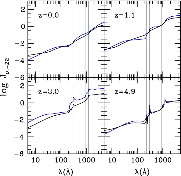
Figure 9. Broadband spectrum of a “quasar-only” cosmic background between 5 Å and 5000 Å at epochs z = 0, 1, 3,and 5. The new models (black curves) are compared with the old results of Paper II (blue curves). The intensity Jν is expressed in units of 10−22 erg cm−2 s−1 Hz−1 sr−1. The vertical thin lines indicate the positions of the H i and He ii Lyα and Lyman limit.
Download figure:
Standard image High-resolution imageThe addition of radiation from galaxies has little effect on the ionizing background at redshifts below 3, as shown in Figure 10, a consequence of our adopted redshift-dependent escape fraction. At higher redshifts the impact is more dramatic: a large boost at 1 ryd is associated with a much sharper He ii sawtooth and He ii absorption edge. As noted above regarding the photoheating rates, this arises because galaxy spectra are truncated at 4 ryd, and the large increase in the H-ionizing emissivity from the early galaxy population is not accompanied by a similar increase at the He ii edge. The net effect is a larger He ii opacity at fixed H i opacity. At z ≳ 5, the He i opacity of the IGM also starts building up (it is negligible at lower redshifts), and a small He i absorption edge can be discerned in the spectrum of the background at 24.6 eV. At z ≳ 3, the sawtooth modulation produced by resonant absorption in the Lyman series of intergalactic He ii (see Figure 11) is clearly a sensitive probe of the nature of the sources that keep the IGM ionized, and may be a crucial ingredient in the modeling of the abundances of metal absorption systems (Madau & Haardt 2009). The analogous sawtooth modulation produced by the H i Lyman series becomes significant above redshift 6 (see Figure 12) and may affect the photodissociation of molecular hydrogen during cosmological reionization (Haiman et al. 1997).
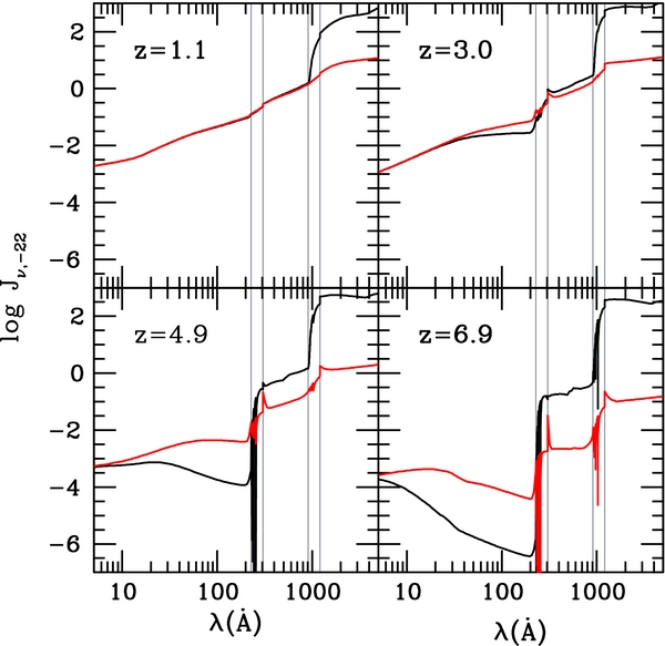
Figure 10. Broadband spectrum of a “quasars + galaxies” cosmic background at redshifts z = 1.1, 3, 4.9, and 5.9 (black curves). The new “quasar-only” model of Figure 9 is plotted for comparison (red curves). The intensity Jν is expressed in units of 10−22 erg cm−2 s−1 Hz−1 sr−1. The vertical thin lines indicate the positions of the H i and He ii Lyα and Lyman limit.
Download figure:
Standard image High-resolution image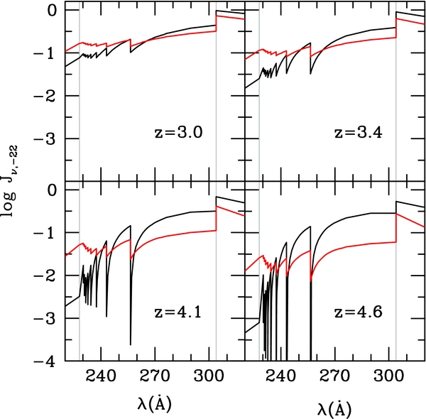
Figure 11. Zoom-in of the “quasars + galaxies” (black curves) and “quasar-only” (red curves) cosmic background spectrum at redshifts z = 3, 3.4, 4.1, and 4.6 showing the sawtooth modulation of the metagalactic flux between 220 and 320 Å produced by resonant absorption in the Lyman series of intergalactic He ii. The vertical thin lines indicate the positions of the He ii Lyα and Lyman limit.
Download figure:
Standard image High-resolution image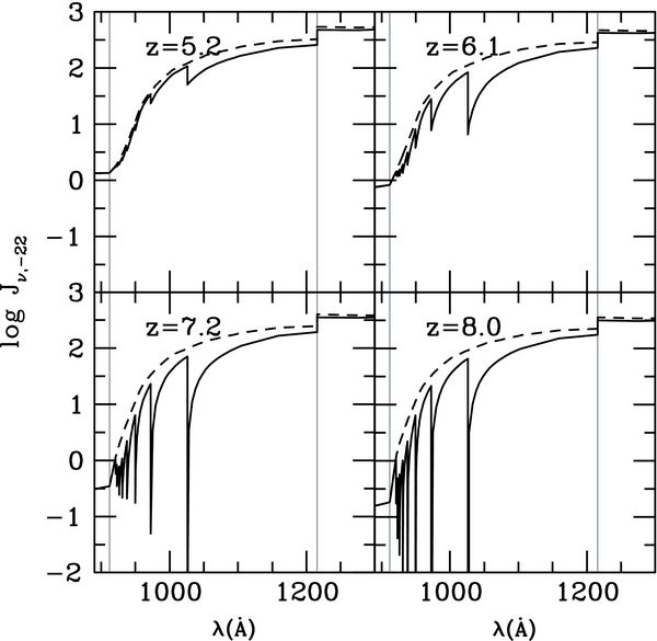
Figure 12. Zoom-in of the “quasars + galaxies” cosmic background spectrum at redshifts z = 5.2, 6.1, 7.2, and 8.0 showing the sawtooth modulation of the metagalactic flux between and 890 and 1300 Å produced by resonant absorption in the Lyman series of intergalactic H i. The vertical thin lines indicate the positions of the H i Lyα and Lyman limit. The dashed line shows the same spectrum without sawtooth for comparison.
Download figure:
Standard image High-resolution imageFigure 13 compares the broadband spectrum of the total extragalactic background light (EBL) from quasars and galaxies, predicted by CUBA at z = 0, with current EBL observations from the mid-IR to the γ-rays.
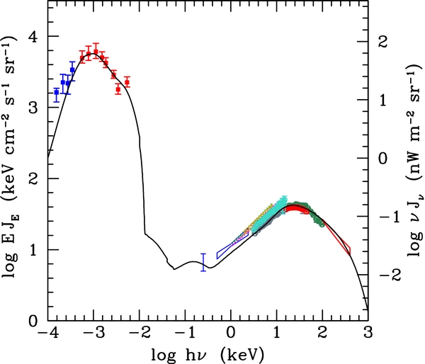
Figure 13. Predicted broadband extragalactic background light, νJν, from quasars and galaxies at z = 0, compared with empirical determinations at different wavelengths. Red points: the optical–near IR EBL from HST and ground-based galaxy counts (Madau & Pozzetti 2000). Blue points: the mid-IR EBL from IRAC-Spitzer galaxy counts (Fazio et al. 2004). The X-ray data points are explained in detail in the caption of Figure 6.
Download figure:
Standard image High-resolution image9.3. A “Minimal Reionization Model”
It is interesting at this stage to use the quasar and galaxy ionizing emissivities of Sections 6, 7, and 8 and track the evolution of the volume filling factors of ionized hydrogen and doubly ionized helium regions in the universe as a function of cosmic time. As shown in Paper III, the volume filling factor of H ii regions,  , is equal at any given instant t to the integral over cosmic time of the number ionizing photons emitted per hydrogen atom by all radiation sources present at earlier epochs,

minus the number of radiative recombinations per ionized hydrogen atom,

Here

with 〈fesc〉 = 1 in the case of quasars, 〈nH〉 = 1.9 × 10⁻⁷(1 + z)3 cm−3 is the mean hydrogen density of the expanding IGM, and 〈trec〉 is the volume-averaged hydrogen recombination timescale,

where αB is the recombination coefficient to the excited states of hydrogen, χ = 1.08 accounts for the presence of photoelectrons from singly ionized helium, and  is the clumping factor of ionized hydrogen. Differentiation yields the H i “reionization equation” of Paper III,

and its equivalent for expanding He iii regions,

where  now includes only photons above 4 ryd (which are mostly absorbed by He ii), and the recombination timescale of doubly ionized helium, 〈trec, He〉, is about six times shorter than the hydrogen recombination timescale if H ii and He iii have similar clumping factors. We will not attempt here to model the reionization of He i, as this occurs nearly simultaneously to and cannot be readily decoupled from that of H i. The reionization equation (1) describes the transition from a neutral universe to a fully ionized one in a statistical way, independently, for a given emissivity, of the emission histories of individual radiation sources; (2) assumes that the mean free path of ionizing photons is much smaller than the horizon, i.e., that they are absorbed before being redshifted below the ionization edge; and (3) includes in the source term only those photons above the Lyman limit that escape into the IGM (〈fesc〉 = 1 in the case of quasars). Photons that are absorbed in loco by dense interstellar gas do not enter in the source term, nor does the interstellar absorbing material contribute to the recombination rate. The volume-weighted clumping factor reflects only the nonuniformity of the ionized low-density IGM, the repository of most of the baryons in the universe, and its use in the recombination timescale is justified when the size of the ionized regions is large compared to the scale of the clumping.
When  (the “pre-overlap” stage), individual ionization fronts propagate from star-forming early galaxies into the low-density IGM. The neutral phase shrinks as
  grows and H ii regions start to overlap. The radiation field remains highly inhomogeneous until the reionization process is completed at the “overlap epoch,”
  , when all the low-density IGM becomes highly ionized. Pockets of neutral gas remain in collapsed systems during the entire “post-overlap” stage (Gnedin 2000) and may manifest themselves as the SLLSs or DLA systems in quasar absorption spectra. We have integrated equation (64) assuming a gas temperature of 2 × 10⁴ K and a clumping factor for the IGM of

This is equal to the expression for C100 (the clumping factor of gas below a threshold overdensity of 100) found at z ⩾ 6 in a suite of cosmological hydrodynamical simulations by Pawlik et al. (2009). These authors found that photoionization heating by a uniform UV background greatly reduces clumping as it smoothes out small-scale density fluctuations, and that the clumping factor at z = 6 is insensitive to the redshift at which the UV background is actually turned on (as long as reheating occurs at ≳ 9). We use an overdensity of 100 to differentiate between dense gas belonging to virialized halos and the diffuse intergalactic gas, and assume that the collapsed mass fraction is small. We also extrapolate Equation (66) down to z ≳ 2, and assume the same clumping factor for H ii and He iii.
The results of this “minimal reionization model” are shown in Figure 14. Cosmological H ii regions driven by star-forming galaxies overlap at redshift 6.7, and the hydrogen in the universe is half-ionized (by volume) at redshift 10. He iii regions driven by quasars overlap much later, at redshift 2.8, and their filling factor is only 4% at redshift 5. These overlap epochs are consistent with the SDSS spectra of z ∼ 6 quasars (Fan et al. 2006b), with numerical simulations of H i reionization (Gnedin & Fan 2006), and with observations of the He ii Lyα forest at z ≲ 3 (see, e.g., Worseck et al. 2011; Shull et al. 2010; Fechner et al. 2006; Heap et al. 2000, and references therein). A simple probe of the reionization history is the integrated optical depth to electron scattering τes, which depends on the path length through ionized gas along the line of sight to the CMB as

(Wyithe & Loeb 2003), where σT is the Thomson cross section. The seven-year WMAP results imply τes = 0.088 ± 0.015 (Jarosik et al. 2011). Our minimal reionization model assumes  and yields an electron scattering opacity to the epoch of reionization of τes = 0.084, in good agreement with the observations.
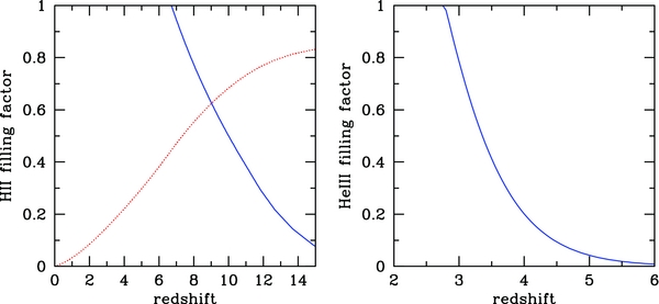
Figure 14. Evolution of the H ii (left panel) and He iii (right panel) filling factors as a function of redshift for our “minimal reionization model” (see the text for details). The dotted curve in the left panel depicts the cumulative electron scattering optical depth of the universe, in units of 10%, as a function of redshift.
Download figure:
Standard image High-resolution imageThe outcome of our minimal reionization model is rather sensitive to the assumed escape fraction of hydrogen-ionizing radiation at early epochs; this exceeds 50% at z ≳ 9 and reaches unity at z = 11.6. Had we assumed a maximum fesc of 50% instead, the same model would yield  at z = 6.2 and τes = 0.06. We also remark that, in the pre-overlap era, the background spectra shown in Figures 9–12 have only a formal meaning, as they describe a space-averaged radiation field that is in reality highly inhomogeneous. Recent spectra taken by the Cosmic Origins Spectrograph on the HST exhibit patchy He ii Gunn–Peterson absorption, with a mean He ii/H i abundance ratio that is 47 ± 42 at 2.4 < z < 2.73 and 209 ± 281 at z > 2.73 (Shull et al. 2010). In the redshift interval 2.4 < z < 2.73, our background spectrum yields a He ii/H i abundance ratio (in the optically thin limit) around 50–70, in good agreement with the observations. The predicted mean He ii/H i ratio increases rapidly toward high redshift to (280, 494, 887, 1615) at z = (3.42, 3.64, 3.87, 4.1) as galaxies start dominating the ionizing emissivity and the spectrum of the UVB steepens. The evolution of the He ii abundance and the fluctuating spectrum of the cosmic UVB in the pre-overlap era will be the subject of a subsequent paper.
9.4. The UVB: Uncertainties
The background spectra computed in the previous section are sensitive to a number of poorly determined input parameters. In this section, we briefly discuss just a few of the uncertainties inherent in our synthesis modeling of the UVB. The left panel of Figure 15 shows the adopted comoving quasar emissivity at 1 ryd (Equation (37)), together with the determinations by Meiksin (2005), Cowie et al. (2009), Bongiorno et al. (2007), Willott et al. (2010), and Siana et al. (2008). The poorly known faint-end slope of the quasar luminosity function at high redshift, incompleteness corrections, as well as the uncertain spectral energy distribution (SED) in the UV, all contribute to the large apparent discrepancies between different measurements.
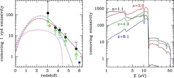
Figure 15. Left: comoving specific emissivity at 1 ryd (in units of 1023 erg s−1 Mpc−3 Hz−1) measured from different quasar surveys. Solid line: the best-fit function in Equation (37). Dashed line: Cowie et al. (2009). Dot-dashed line: Bongiorno et al. (2007), using a 912 Å to 4400 Å flux ratio of 0.31. Filled circles: Meiksin (2005), PLE model. Empty circles: Meiksin (2005), PDE model. Empty star: Siana et al. (2008). Filled square: Willott et al. (2010) at z = 6. Right: comoving galaxy emissivity per logarithmic bandwidth (in units of 1039 erg s−1 Mpc−3) escaping into the IGM, as a function of photon energy, at four different redshifts. Note the large, time-evolving break at 13.6 eV.
Download figure:
Standard image High-resolution imageThe escape fraction of ionizing radiation that leaks into the IGM and its unknown redshift evolution is the major source of uncertainty in the determination of the galaxy contribution to the UVB. To better gauge the impact of this parameter on our synthesis model, we show in the right panel of Figure 15 the spectrum of the comoving galaxy emissivity at four different epochs. The relatively large leakage of LyC photons assumed at early times is a crucial ingredient of our “minimal reionization model,” which yields an optical depth to Thomson scattering in agreement with WMAP results. A smaller escape fraction at high redshifts would lead to too-late reionization, while a significantly larger escape fraction at lower redshifts would produce a hydrogen photoionization rate that appears to be too high compared to the observations (see Figure 8).
We have also checked that, for a given IMF, uncertainties in the stellar population synthesis technique are relatively small. Figure 16 shows the emission rate of hydrogen-ionizing photons for an SSP, calculated as a function of age with the GALAXEV models of Bruzual & Charlot (2003), the Starburst99 models of Leitherer et al. (1999), and the FSPS models of Conroy et al. (2009). While the three packages use different stellar evolution tracks and spectral libraries, the total number of ionizing photons emitted agrees to within 10%. The figure also illustrates the significant effect of stellar metallicity: an SSP of metallicity 1/50 of solar emits 60% more hydrogen-ionizing photons over its lifetime than a solar metallicity SSP (Salpeter IMF, GALAXEV package).
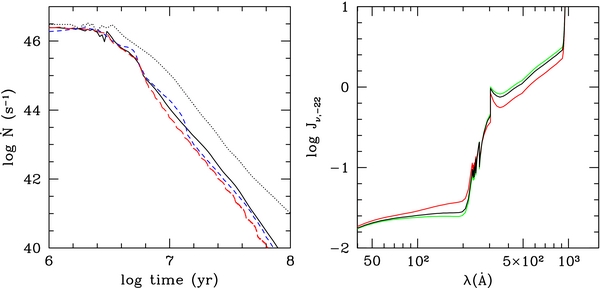
Figure 16. Left: emission rate of hydrogen-ionizing photons for an SSP of total mass 1 M☉, Salpeter IMF, and solar metallicity, as a function of age. Solid line: results from the GALAXEV package of Bruzual & Charlot (2003). Long-dashed line: same for Starburst99 (Leitherer et al. 1999). Short-dashed line: same for the FSPS package of Conroy et al. (2009). Dotted line: same as the solid line, but for a metallicity 1/50 of solar. Right: uncertainties in the broadband spectrum of the “quasars + galaxies” UVB at redshift 3. Black line: our fiducial model. Green line: a model with a slope of β = 0.2 in the column density distribution of LLSs. Red line: same for β = 1.0. The intensity Jν is expressed in units of 10−22 erg cm−2 s−1 Hz−1 sr−1.
Download figure:
Standard image High-resolution imageFinally, we address the effect of a change in the effective opacity of the IGM. In our parameterization, the shape of the  distribution over the column density range of the LLSs is adjusted at every redshift for continuity with the SLLSs. As detailed in Section 3, this procedure yields the slopes β = 0.47, 0.61, 0.72, 0.82 at redshifts z = 2, 3, 4, 5, respectively. To gauge how an uncertainty in
  translates into an uncertainty in the UVB, we have run CUBA with the fixed values of β = 0.2 and β = 1 in the column density interval
  . The resulting UVB at z = 3 is shown in the right panel of Figure 16. Compared to our fiducial model, the flat β = 0.2 distribution generates a hydrogen photoionization rate (
 ) that is 29% lower and a He ii photoionization rate (
 ) that is 22% higher. This is because a larger opacity at 1 ryd from the LSSs results in a harder background spectrum, which in turn produces a smaller He ii opacity at 4 ryd. Conversely, in the steep β = 1 case,
  increases by 8% and
  decreases by 10%. Note, however, that the former model would significantly underestimate the 1 ryd photon mean free path compared to the measurements of Prochaska et al. (2009).
10. SUMMARY
In this paper, we have presented improved synthesis models of the evolving spectrum of the UV/X-ray diffuse background, updating and extending our previous results. Five new main components have been added to our cosmological radiative transfer code CUBA and discuss in details: (1) the sawtooth modulation of the background intensity from resonant line absorption in the Lyman series of cosmic hydrogen and helium; (2) the X-ray emission from the obscured and unobscured quasars that gives origin to the XRB; (3) a piecewise parameterization of the distribution in redshift and column density of intergalactic absorbers that fits recent measurements of the mean free path of 1 ryd photons; (4) an accurate treatment of the absorber photoionization structure, which enters in the calculation of the helium continuum opacity and recombination emissivity; and (5) the UV emission from star-forming galaxies at all redshifts. The full implications of our new population synthesis models for the thermodynamics and ionization state of the Lyα forest and metal absorbers will be addressed in a subsequent paper. Here we have provided tables of the predicted H i and He ii photoionization and photoheating rates for use, e.g., in cosmological hydrodynamics simulations of the Lyα forest, a new metallicity-dependent calibration to the UV luminosity density-star formation rate density relation, and presented a “minimal cosmic reionization model” in which the galaxy UV emissivity traces recent determinations of the cosmic history of star formation, the luminosity-weighted escape fraction of hydrogen-ionizing radiation increases rapidly with look-back time, the clumping factor of the high-redshift IGM follows recent determinations of hydrodynamic simulations that include the effect of photoionization heating, and Population III stars and miniquasars make a negligible contribution to the metagalactic flux. The model has been shown to provide a good fit to the hydrogen-ionization rates inferred from flux decrement and quasar proximity effect measurements, to predict that cosmological H ii (He iii) regions overlap at redshift 6.7 (2.8), and to yield an optical depth to Thomson scattering, τes = 0.084, which is in agreement with WMAP results.
Our new background intensities and spectra are sensitive to a number of poorly determined input parameters and suffer from various degeneracies. Their predictive power should be constantly tested against new observations. We are therefore making our redshift-dependent UV/X emissivities and CUBA outputs freely available for public use at http://www.ucolick.org/~pmadau/CUBA.
We have benefited from many informative discussions with A. Boksenberg, S. Charlot, A. Comastri, C.-A. Faucher-Giguère, M. McQuinn, J. Prochaska, C. Scarlata, and G. Worseck. Support for this work was provided by NASA through grant NNX09AJ34G and by the NSF through grant AST-0908910 to P.M., and by the MIUR, PRIN 2007 to F.H.
APPENDIX: THE IONIZATION AND THERMAL STATE OF INTERGALACTIC ABSORBERS
In this Appendix, we describe the numerical calculations of the ionization structure of individual absorbers outlined in Section 4. We approximate each absorber as a semi-infinite slab with uniform hydrogen density nH and thickness equal to its Jeans length,

(Schaye 2001; Faucher-Giguère et al. 2009), where the adiabatic index and mean molecular weight for a monoatomic, fully ionized gas of primordial composition are γ = 5/3 and μ = 0.59, respectively, and T4 is the gas temperature in units of 104 K. The gas mass fraction is set at its universal value, fg = Ωb/ΩM = 0.16. Each slab model provides, given the gas density nH and an external isotropic radiation field Jν, the columns  ,
,  , and
, and  . The slab geometry reduces the local radiative transfer to a two-dimensional problem (see Figure 17). Setting μ ≡ cos θ, where θ is the angle between the incident ray and the normal at the slab, the specific intensity Iν(x, μ) at coordinate x within the slab is given by the following implicit solution to the radiative transfer equation:

Here, jν is the recombination radiation emission coefficient along the ray,

is the optical depth normal to the slab, and the sum is to be taken over all relevant species. Integration over solid angle yields the local specific brightness 
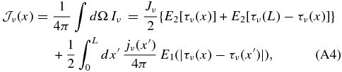
where E1 and E2 are the first- and second-order exponential integral functions, respectively. The symmetry of the problem allows us to study just half of the slab, as for all ions n(x) = n(L − x). With this in mind, we can rewrite the external contribution to  (the first term on the right-hand side of Equation (A4)) as

(0 < x < L/2), and the contribution of recombinations (the second term on the right-hand side of Equation (A4)) as
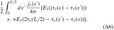
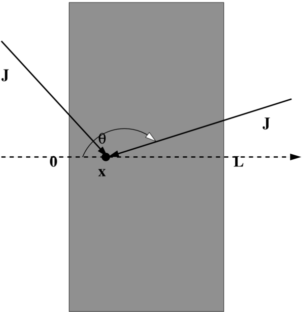
Figure 17. Slab approximation for individual absorbers: a plane-parallel slab of thickness L illuminated by an isotropic external radiation field J.
Download figure:
Standard image High-resolution imageThermal equilibrium in the absorbers is obtained by balancing photoionization heating with a number of different energy loss mechanisms: free–free, collisional excitations and ionizations, recombinations, Compton cooling against the cosmic microwave background, and adiabatic cooling from cosmic expansion. The photoheating rate (per ion) is given by

where hνi is the ionization potential of species i. The equation of thermal equilibrium can then be written as

where Λc is the atomic cooling rate and the last term accounts for adiabatic cooling. Our treatment of the thermal state of cosmological absorbers is oversimplified in two aspects: (1) the lowest density IGM is not in thermal equilibrium and (2) dense quasar absorbers do not expand with the Hubble flow. We find, however, that (1) adiabatic cooling is never important for absorbers with  cm−2, so the inclusion of this process does not alter the thermal balance in this column density regime and (2) in low the density, optically thin IGM, the functions
  and (to a lesser extent)
  are independent on gas temperature, and hence the assumption of thermal equilibrium should not affect our results.
The ionization and thermal structure of the slab, for a given Jν and nH, are solved by iteration. We start by assuming an almost fully ionized slab at T = 104 K and compute the ionization rates Γi setting the recombination emissivity to zero. We then solve for the ionization structure within the slab, compute updated ion fractions and opacities, and evaluate new ionization rates including recombination radiation. The process is iterated until convergence to better than 0.1% is obtained at every point of the slab. At each iteration the size of the slab is changed accordingly to the Jeans criterion (Equation (A1)).
Footnotes
- 3
In this section, we use the notation ρν(z) ≡
ν(z)/(1 + z)3, i.e., the term luminosity density is synonymous with comoving specific emissivity.