ABSTRACT
We examine variations of the stellar initial mass function (IMF) in extreme environments within the formalism derived by Hennebelle & Chabrier. We focus on conditions encountered in progenitors of massive early-type galaxies and starburst regions. We show that, when applying the concept of turbulent Jeans mass as the characteristic mass for fragmentation in a turbulent medium, the peak of the IMF in such environments is shifted toward smaller masses, leading to a bottom-heavy IMF, as suggested by various observations. In very dense and turbulent environments, we predict that the high-mass tail of the IMF can become even steeper than the standard Salpeter IMF, with a limit for the power-law exponent α ≃ −2.7, in agreement with recent observational determinations. This steepening is a direct consequence of the high densities and Mach values in such regions but also of the time dependence of the fragmentation process, as incorporated in the Hennebelle–Chabrier theory. We provide analytical parameterizations of these IMFs in such environments to be used in galaxy evolution calculations. We also calculate the star-formation rates and the mass-to-light ratios expected under such extreme conditions and show that they agree well with the values inferred in starburst environments and massive high-redshift galaxies. This reinforces the paradigm of star formation as being a universal process, i.e., the direct outcome of gravitationally unstable fluctuations in a density field initially generated by large-scale, shock-dominated turbulence. This globally enables us to infer the variations of the stellar IMF and related properties for atypical galactic conditions.
1. INTRODUCTION
Stars form from the collapse of prestellar dense cores, themselves forming in the overdense regions (clumps) of large molecular gas reservoirs, called giant molecular clouds (GMCs). The generic properties of the prestellar core mass function (CMF) and of the resulting stellar initial mass function (IMF) are intrinsically associated with the general properties of these clouds. Various determinations of the IMF in the Milky Way (MW) Galaxy, disk, bulge, and nearby star-forming regions and young clusters suggest essentially no or very little variation, with all of the inferred IMFs being consistent within some expected scatter with the same underlying Chabrier (2005) IMF5 (Chabrier 2003, 2005; Andersen et al. 2008; Bastian et al. 2010). Similarly, mass-to-light (M/L) ratio determinations in spiral galaxies are also consistent with this same IMF (e.g., Portinari et al. 2004; van Dokkum & Conroy 2010; Brewer et al. 2012; Tortora et al. 2013, 2014). In contrast, there is now growing evidence from various observations that the IMF in massive elliptical early-type galaxies (ETGs) differs from the previous one, being more “bottom heavy” and revealing a larger fraction of low-mass stars compared to MW-like environments. Spectroscopic observations indeed show a marked increase in the strengths of various spectral line absorption features with velocity dispersions in the σ = 100–300 km s−1 range, pointing to the existence of a large population of M dwarf stars and thus a more bottom-heavy IMF compared to the MW (van Dokkum & Conroy 2010, 2012; Conroy & van Dokkum 2012a, 2012b; Smith et al. 2012; Spiniello et al. 2012, 2014; Ferraras et al. 2013; La Barbera et al. 2013; Goudfrooij & Kruijssen 2013). Furthermore, constraints from observed stellar kinematics and gravitational lensing confirm that massive ETGs have large mass-to-light ratios compared to other galaxies (e.g., Treu et al. 2010; Thomas et al. 2011; Cappellari et al. 2012, 2013; Sonnenfeld et al. 2012; Conroy et al. 2013; Dutton et al. 2013a, 2013b; Barnabè et al. 2013; Tortora et al. 2013, 2014). Combined with the former spectroscopic diagnostics, these results suggest that this large mass arises from an unusually large low-mass star population rather than from a population of remnant stars. Further valuable spectroscopic information is the signature of enhanced [α/Fe] abundance ratios with increasingly large velocity dispersion in the spectra of massive ETGs (Thomas et al. 2011; Conroy & van Dokkum 2012a, 2012b; Conroy et al. 2014), suggesting that the IMF evolves from a Chabrier-like one at abundance ratios close to solar to a more bottom-heavy one for highly α-enhanced populations. Under the conventional assumption that these ratios reflect the star-formation timescale, with higher values corresponding to shorter timescales, all of these observations suggest that galaxies harboring α-enhanced stellar populations, formed in rapid and intense starbursts, tend to generate a larger population of low-mass stars than galaxies with extended star-formation histories. The progenitors of massive ETGs, formed in the early universe, are the emblematic representation of such structures.
The consistent picture that seems to emerge from all of these data is that the IMF is not completely “universal” but varies from MW-like for spiral galaxies, with moderate velocity dispersion formed at low redshift (z ≲ 2) with “quiescent” star-formation histories, to Salpeter-like or even steeper over the entire stellar regime for massive star-forming galaxies, with velocity dispersion σ ≳ 200 km s−1, in which stars formed very rapidly in a “burst” mode at early epochs. As discussed in Section 3, massive ETGs are indeed supposed to be the result of the merging of compact structures formed within large gas inflows in the early universe, exhibiting presumably more extreme star-formation conditions, gas mean density, and velocity dispersion than the ones prevailing in the MW. In the local universe, extreme star-forming conditions, resulting from gas-rich mergers, also prevail in starburst environments like the central parts of ultraluminous infrared galaxies (ULIRGs; e.g., Kartaltepe et al. 2012).
In this paper, we explore this issue by examining the dependence of the IMF on the environment, i.e., the cloud gas temperature, mean density, and turbulent properties, within the framework of the Hennebelle & Chabrier (hereafter HC; 2008, 2009, 2013) analytical theory of the IMF. This “gravoturbulent” picture of star formation indeed predicts variations of the IMF with the level of turbulence, in contrast to the standard, purely gravitational star-formation scenario, and might naturally explain the aforementioned variations. It should be noted that Hopkins (2013) recently explored this issue with a different formalism. Besides the fact that it is important to verify whether different theories yield similar conclusions, we expand upon Hopkins' results in several ways: first by including the time dependence of the IMF in our formalism, second by calculating the inferred star formation rates (SFRs) and mass-to-light ratios in such extreme environments, and third by providing analytical parameterizations of the Chabrier IMF relevant for such conditions. The paper is organized as follows. We first derive in Section 2 the relations between the normalizations of Larson relations at a cloud scale and those at a galactic scale so that the star-forming cloud properties can be inferred directly from the ones of the host galaxy. In Section 3, we examine the particular conditions prevailing in massive ETG progenitors and how they modify the aforementioned normalizations. In Section 4, we summarize the Hennebelle–Chabrier theory and highlight its main predictions relevant to the present study. In Section 5, we calculate the IMFs characteristic of extreme star-forming conditions, for which we provide analytical parameterizations. The SFRs and M/L ratios obtained with these different IMFs are calculated in Section 6 and 7, respectively, and Section 8 is devoted to the conclusion.
2. FROM CLOUD TO GALACTIC PROPERTIES
2.1. Larson Relations
As mentioned above, stars form inside overdense regions, usually denominated “clumps,within giant molecular gas clouds.6 We thus consider the properties of the gas in a population of star-forming clumps or clouds formed in a given host galaxy. In the MW, star-forming clumps or clouds are observed to follow the so-called Larson (1981) scaling relations between the cloud H2 mean number density  or three-dimensional (3D) velocity dispersion Vrms (which includes both rms and thermal fluctuations) and its size Lc within a domain ranging from ∼one to several hundreds of parsecs:


These relations correspond to the nearly equilibrium state of molecular clouds immersed in an ambient medium of constant pressure P (Chièze 1987). As obvious from these equations, d0 and V0 define the density and velocity dispersion normalization conditions at the 1 pc scale. Observed values in GMCs in the Galaxy give d0 ∼ 3 × 103 cm−3 and V0 ∼ 0.8–1.0 km s−1.
For a homogeneous self-gravitating cloud of mass Mc and size Lc, the (molecular) gas surface density and pressure read


where  , with μ = 2.33 for a cosmic composition and mh = 1.66 × 10⁻²⁴ g, denotes the cloud H2 mean mass density and where we have assumed that essentially all of the gas in GMCs is in molecular form. A condition of constant pressure thus yields ηd = 1 in Equation (1). Observations rather suggest ηd ∼ 0.7–1.0 (Hennebelle & Falgarone 2013) due to the nonhomogeneous, arguably fractal nature of GMCs, while the exponent η is found to be η ∼ 0.4–0.5. Strikingly, these scaling relations, illustrating the connection between the properties within a cloud and its ambient medium, are observed to be remarkably universal, not only under MW-like conditions but also in completely different environments like high-redshift, star-forming galaxies (e.g., Swinbank et al. 2011) or the MW central molecular zone (CMZ; Shetty et al. 2012; Kruijssen & Longmore 2013). The exponents in these systems remain similar. The “universality” of the linewidth–size relation within star-forming GMCs and the fact that it holds over a large range of spatial scales, in particular, suggests that the underlying physical processes driving the interstellar medium (ISM) dynamics are “universal,pointing to supersonic turbulence, and provides evidence for large-scale (low spatial frequencies, >10 pc) turbulent driving (Heyer & Brunt 2004; Kritsuk et al. 2013). This picture is consistent with GMCs forming on large scales from colliding flows or global galactic disk instabilities and inheriting the turbulent properties of these large-scale motions. One can indeed relate the value of the exponent η to the (3D) index n of the turbulence velocity power spectrum,
 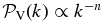 , as (e.g., Hennebelle & Chabrier 2008)

Various simulations of compressible (magneto)turbulence (e.g., Kritsuk et al. 2007, 2013; Molina et al. 2012) suggest a value n ∼ 3.8, which yields η ∼ 0.4, the observed value.
2.2. Normalization on Large Scales
It is useful to link the dynamical properties of the gas within star-forming clouds, as given by Equation (2), the relevant scale for the stellar IMF, to the ones of the host galaxy, characterized by a typical length scale rd, generally defined as the typical gas scale height rd ∼ h. Such a limit between clouds and the surrounding ISM on large scales, however, is rather ill-defined, both theoretically and observationally, and necessarily retains large uncertainties. The easiest way to proceed is simply to extend the scaling relation (2) up to scales Lc ∼ h, typical of the largest GMCs, by assuming that the largest turbulence injection scale is Li ∼ Lc ∼ h. The velocity dispersion of the star-forming gas in GMCs at the galactic characteristic scale r ∼ h is thus the one given by the condition of a Toomre marginally stable disk (Q ∼ 1) with gas average volume density ρg and midplane surface density Σ0 = Σg(z = 0) = 2hρg, corresponding to a gas mass Mg(r) ≈ πΣ0(r)r2. This assumption, which is in substance the one adopted by Hopkins (2012a), seems to be generally observationally verified from normal disk to starburst galaxies (e.g., Downes & Solomon 1998). The big leap behind this procedure, however, is the assumption that the dynamical properties of the gas in star-forming clumps are only marginally affected by the transition from the H i to H2 gas or by large-scale gradients, so the atomic and molecular gas belong to the same turbulent cascade from galactic scales to cloud scales. Under such an assumption, the gas velocity dispersion versus size relation for star-forming clumps smoothly decreases from the largest possible turbulent scale, r = Li ∼ h, to scales relevant for star formation and the IMF, r ≪ h, while the galactic rotational shear,  , where
  is the disk epicyclic frequency and Ω = vrot/r is its angular frequency, dominates on scales of r ≫ h (e.g., Hopkins 2012a):

with ν(r) ≃ Vrms(r) for r ≪ h and 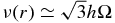 for r ≳ h. Vertical hydrostatic equilibrium for the gas disk at scale r ≳ h implies
  . As mentioned above, this corresponds to the general scaling relation for the velocity dispersion in a marginally stable disk (Q(r) ∼ 1) on scale r ∼ h, which corresponds to the most unstable scale in a turbulent disk. This leads to the scaling relation at r ∼ h (within geometrical factors of the order of a few):
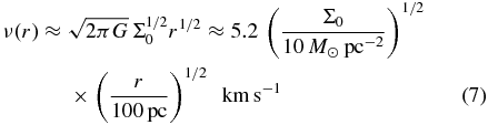

Equating Equations (8) and (2) at scale r ∼ Lc ∼ h provides the normalization condition of Equation (2), which gives a measure of the typical amplitude of turbulent motions at the 1 pc scale, in terms of the one at scale h:
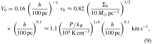
where νh ≡ ν(h) and the numerical factors have been evaluated for η = 0.4.7
Note that, in the above estimates, we have assumed for the sake of simplicity that the disk consists entirely of molecular gas in GMCs. Considering that these latter only contain a fraction of the disk surface density will basically introduce a correcting factor  in the above expressions, changing Σ0 by
  . Assuming that most of the galaxy molecular gas is collected into large bound GMCs of size ∼100 pc,
  is essentially the galaxy molecular gas fraction. For MW typical conditions (Σ0)MW ≃ 20 M☉ pc−2, (P/kB)MW ≃ 1.5 × 10⁴ K cm−3, Equation (9) recovers the typical value for V0 mentioned in the previous section.
We can also infer the density normalization. Assuming again (e.g., Krumholz & McKee 2005) that the mass of the most massive star-forming clouds is approximately the critical Toomre mass in the galactic disk (which is similar to the two-dimensional Jeans mass for Q ∼ 1, with the wavelength of the fastest growing mode LJ = ν2/πGΣg ∼ h), i.e.,  (again within numerical or geometrical factors on the order of a few), one gets, at scale r ∼ LJ ∼ h,
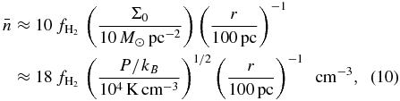
and thus, using Equation (1),
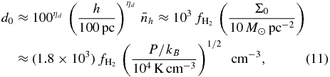
where  and where we have used ηd ∼ 1. This yields a mass–size relation for the GMCs (assuming nearly spherical clouds):
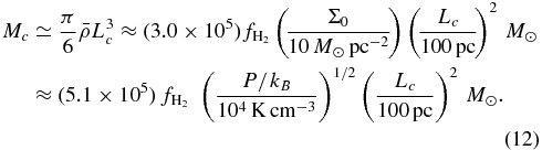
Equations (9) and (11) enable us to relate the normalizations of the cloud mean properties at 1 pc in Equations (1) and (2) to the ones at the galactic scale (h ∼ 100 pc). In order to avoid the uncertainties in the various numerical coefficients, these relations can be used relative to the values in the MW:
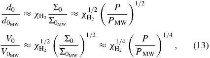
where  is the ratio of the fraction of molecular gas surface density in the galaxy under consideration compared with the MW value, a parameter of order unity.
As mentioned above, these relations implicitly assume that the Larson relations reflecting the cloud mean densities and dynamical properties apply all the way through from clump scales to galactic scales, regardless of possible large discontinuities either in mean density or turbulence properties between star-forming GMCs and the surrounding ISM. Such an approximation is probably of questionable validity for nearby galaxies like the MW where GMCs are discrete, generally gravitationally bound entities much denser than the surrounding ISM (typically n ∼ 100 cm−3 versus ∼1 cm−3) and the ISM is dominated by atomic gas. Starburst and high-z massive galaxies, however, are characterized by high surface densities and a larger molecular gas fraction (e.g., Daddi et al. 2010), so the ISM is a rather continuous star-forming, turbulent medium with a more modest (≲ 10 or so) density contrast with the GMCs (e.g., Dekel et al. 2009; Ceverino et al. 2010). Moreover, the star-forming clumps in starburst environments are confined by a nearly constant bounding pressure during their star-formation history, allowing the use of the Larson relations (Chièze 1987). Therefore, the above relations should provide reasonable estimates of star-forming cloud conditions in various environments, expressed in terms of those typical of the MW.
In conditions such as those leading to the formation of massive ETG progenitors, the external pressure at the surface of the GMC is directly related to the kinetic pressure of the infalling (circumgalactic) gas,  . In a nearly virialized gas disk, the infall velocity is on the order of the virial velocity, vinf(r) ≈ Vrot(r) = (GM/r)1/2 (Genel et al. 2012). However, although the inflow velocity of cold gas streams is indeed found to be close to the virialization velocity of the isothermal halo for local spiral galaxies (e.g., Dekel et al. 2009), this is unlikely to be the case for high-z, massive clumpy starburst galaxies such as those leading to the formation of ETG progenitors. This lack of equilibrium condition prevents a precise determination of the correlation between gas velocity and virial velocity, in contrast to the stellar component, ΔV⋆∝Vrot.
On the other hand, some (potentially large) fraction ξ of the infall kinetic energy is expected to be converted into turbulent kinetic energy, leading to a ram pressure,  , at the surface of the star-forming clouds (e.g., Bournaud et al. 2011; Genel et al. 2012). The turbulent dissipation rate within the star-forming clouds,
  , where
  is the typical crossing time within the cloud, is thus related somehow to the gas accretion rate,
  , with some geometrical factor of the order of unity:

Therefore, at least part of the gas dispersion velocity in the star-forming clouds is expected to correlate directly with the gas inflow rate on the galaxy.
3. MASSIVE EARLY-TYPE GALAXIES AND EXTREME STARBURST ENVIRONMENTS
In the modern paradigm of structure formation, most of the stars that have ended up today in the cores of massive (M⋆ ≳ 1010 M☉) ETGs formed in small, dense, gas-rich primordial star-forming galaxies, at redshifts between z ∼ 3 and 5, i.e., within a rather short timescale Δt ∼ 1–2 Gyr (see, e.g., de Lucia & Blaizot 2007; Wilman et al. 2013; Naab et al. 2007; Barro et al. 2013). As mentioned in Section 1, measurements of enhanced α-element abundances in the spectra of these galaxies indeed suggest a star-formation timescale of a few megayears (Thomas et al. 2005; Conroy et al. 2014). Hence, star formation in the progenitors of massive ETGs presumably occurred more in burst modes than in gradual “disk” modes typical of star-forming galaxies at lower redshift. Then these primordial structures continued to grow, mainly through dry (gas-poor), minor merger events, to eventually lead to the formation of the massive ETGs observed today, without producing significant new stars (see references above). The early phases of star formation in massive ETG progenitors thus involve violent dynamical dissipational processes, such as gas-rich mergers or dynamical instabilities fed by strong infalling gas flows from the intergalactic medium (IGM), that induce compact starbursts in the central regions. Gas consumption into stars in the central starburst, ram pressure on dust grains, or outflows driven by stellar or active galactic nucleus feedback mechanisms then quench star formation on very short (dynamical) timescales, and the galaxy then evolves passively. Therefore, according to this paradigm, star formation in massive ETG progenitors occurred throughout bursts in dense/compact galaxies and was driven primarily by intense, cold gas accretion events, originating from gas streams along the filaments of the cosmic web, efficiently forming stars centrally rather than in an extended disk (e.g., Genel et al. 2012). The IMF was imprinted during these early phases of intense gas-rich accretion and remained barely affected afterward, conditions quite different from the ones prevailing in quiescent MW-like spiral galaxies.
3.1. Density
As just mentioned, the high-redshift (z ≳ 2) progenitors of massive ETGs are much more compact, with sizes smaller by a factor of ∼six, than bulges or spiral galaxies of similar stellar mass in the local universe (Barro et al. 2013; Williams et al. 2014). The combination of high masses and small sizes results in extremely high densities. Similar conditions are expected in the central regions of massive elliptical galaxies that are thought to form in compact starbursts (e.g., Diamond-Stanic et al. 2012). The average gas surface densities in star-forming clouds in starburst galaxies range from Σg ∼ 103 to 105 M☉ pc−2 (Turner et al. 2000; van Dokkum et al. 2008), compared to a typical range ∼1 to 102 M☉ pc−2 within a typical MW disk GMC (Kennicutt 1998; Bryant & Scoville 1999). After Equation (4), such high densities correspond to interstellar ISM pressures as high as P/kB ≳ 107–1011 K cm−3, compared to P/kB ∼ 104 K cm−3 for the typical MW ISM pressure.
According to the relations derived in Section 2.2, such a dense and highly pressurized ISM leads to the formation of massive (up to ∼1010 M☉) and dense star-forming regions, a factor of ≳ 104 × higher than the largest characteristic mass of GMCs in the MW (e.g., Elmegreen et al. 2007; Swinbank et al. 2012). Using Equations (11) and (13), the density normalization at 1 pc is expected to reach values as high as d0 ∼ 106 cm−3 in such starburst regions. This means that, under such high-pressure conditions, the molecular gas can be more than ∼1000 times denser at all scales than the gaseous star-forming clumps in the MW. Indeed, the compact central starbursts and central regions of ULIRG-like galaxies (gas-rich mergers) have characteristic gas densities that are 102–104 times higher than the average for normal disks, with the dominant gas mass fraction lying at densities n(H2) ≳ 105 cm−3 (Gao & Solomon 2004; Diamond-Stanic et al. 2012). Extreme starburst regions like Arp 220 are larger than ordinary GMCs but are filled with molecular gas at a density usually found only in small cloud cores (Downes & Solomon 1998).
3.2. Velocity Dispersion
As mentioned above, the most admitted explanation for the rapid and significant early mass growth of the progenitors of the most massive ETGs involve violent dynamical processes, such as repeated gas-rich (“wet”) mergers or strong accreting gas flows at high redshift, with most of their stellar mass being formed by z ∼ 3. Accretion rates onto the galaxy from the IGM reach values as large as  , to be compared with
  for the MW (e.g., Dekel et al. 2009; Ceverino et al. 2010; Klessen & Hennebelle 2010). These accreting flows produce a highly turbulent velocity field that pervades the whole region as the gas is entrained into the flow. Globally, the combined effects of large accretion rates, larger densities, and higher pressures relative to the local ISM all yield a systematic enhancement of turbulent velocities at all scales. According to Equations (9) and (14), we expect a factor of ∼5–10 increase in the normalization factor V0 at the 1 pc scale, yielding values as high as V0 ∼ 10 km s−1 under the aforementioned conditions. The CMZ, for instance, characterized by larger ambient pressure and larger densities and temperatures than the local ISM, is found to exhibit velocity dispersions systematically higher, resulting in a scaling coefficient approximately five times larger than for GMCs in quiescent environments like the standard MW clouds (e.g., Swinbank et al. 2011, Figure 6; Shetty et al. 2012, Figure 8). High-redshift galaxies are indeed characterized by a considerably higher degree of internal turbulence than present-day galaxies of comparable mass (Genzel et al. 2008).
3.3. Temperature
The temperature of the gas in a molecular cloud depends on many different physical processes. To the best of our knowledge, detailed calculations have not been conducted for ETG progenitors or starburst environments, so it is difficult to infer the typical gas temperature under such conditions. This latter, however, is intuitively expected to be significantly larger than the typical T ∼ 10 K value representative of relatively quiescent, low-density, star-forming molecular clouds. First of all, as mentioned above, star formation in the progenitors of present ETGs is expected to have occurred through an initial burst at z ∼ 5, yielding a minimum background temperature of about ∼20 K. Second of all, the predominance of gas compression due to gas inflows and shock-dominated turbulent motions yields a large compressional heating rate ( ). At a first order, the dissipation of this kinetic energy into thermal energy will raise the gas temperature, even though part of this energy will be radiated away. In extreme starbursts like those in low-redshift ULIRGs, the infrared emission peaking at wavelengths ∼60–100 μm reveals dust heated at temperatures Td ∼ 60–70 K in molecular clouds (Downes & Solomon 1998; Greeve et al. 2009). At the high densities typical of the regions of interest,
  , gas–dust energy exchange becomes quite efficient, so the kinetic temperature of the (thermally coupled) gas reaches similar values. Of course, what matters is the temperature of the gas before star formation sets in, so the comparison with ULIRGs might be questionable. The consequences of the uncertainties in the gas temperature on the IMF will be addressed in Section 5.1.
In the calculations below, we will examine the impact of such high density, pressure, temperature, and velocity dispersion conditions upon the IMF. A word of caution, however, is necessary. Despite the support provided by the above general analysis, our assumption that the physical conditions in ETG progenitors and in starburst environments are similar could be questioned. The temperature determination, for example, is particularly uncertain. The vicinity of an H ii region, common in spiral galaxies as opposed to ellipticals, or of a black hole, for instance, might heat up the gas significantly, thereby decreasing the cloud typical Mach number ( ). Dense, high-pressure environments thus do not necessarily imply highly turbulent conditions. These uncertainties must be borne in mind when trying to characterize ETG progenitor conditions.
4. HENNEBELLE–CHABRIER THEORY. GENERAL FORMALISM AND MAIN FEATURES.
Recently, Hennebelle & Chabrier (2008, hereafter HC08) have developed an analytical theory of the IMF, extending the Press & Schechter formalism developed in cosmology for linear density fluctuations to the gravoturbulent picture of star formation, characterized by highly nonlinear fluctuations. This theory successfully reproduces within the same framework the observed distribution of unbound CO clumps and of gravitationally bound prestellar cores.8 Both the clump and the core mass functions only depend on one single parameter, namely the index of the log density and velocity power spectra of turbulence. This index is indeed found to be similar for both spectra in simulations of shock-dominated turbulence in the explored range of Mach values, with a characteristic (3D) value n′ ≃ n ≃ 3.8 (e.g., Kritsuk et al. 2007) between the Kolmogorov and Burgers values. In the HC formalism, the normalization and the width of the IMF are then entirely determined by the characteristic conditions of the parent molecular cloud, mean density  , temperature T, and large-scale Mach number
  , where CS ≃ 0.19 (T/10 K)1/2(μ/2.33)−1/2 km s−1 is the sound velocity.
In a subsequent paper, Hennebelle & Chabrier (2009, hereafter HC09) took into account the thermodynamics of the gas and showed that it has a significant impact on the low-mass part of the spectrum. More recently, the same authors have included the time dependence in their theory, extending the calculations to an analytical derivation of the SFR (Hennebelle & Chabrier 2011a, 2013, hereafter HC11 and HC13). This leads to some modifications of the low-mass part of the IMF compared with the static theory and predicts SFRs in very good agreement with the observed values in MW molecular clouds (see HC13).
Although alternative IMF theories have been suggested (see, e.g., Hennebelle & Chabrier 2011b; Offner et al. 2014, for recent reviews), the most achieved one, besides HC, is the one recently derived by Hopkins (2012a), based on the so-called excursion set formalism also used in cosmology. Both the HC and Hopkins theories rely on the concept of structure (cloud or core) formation being induced by density fluctuations,  , induced by the small-scale dissipation of large-scale supersonic turbulence. The random field of density fluctuations is thus given by the probability density function (pdf; i.e., power spectrum) of turbulence. For isothermal (magnetized or nonmagnetized) turbulence, this latter has been found in many studies to be well reproduced by a lognormal form (see, e.g., Vázquez-Semadeni 1994; Federrath 2013 and references therein), i.e., a Gaussian field in logarithm of the density, characterized by a variance σ(δ). We stress, however, that both HC and Hopkins theories remain valid for any choice of the pdf, even though a lognormal form greatly simplifies the calculations. Smoothed at scale R, the random field of fluctuations
  is thus given by


Here Wk is a window function, chosen to be the sharp-k space-truncated function. Various simulations of supersonic turbulence (see above references) yield for the variance of the unsmoothed density field, σ0,

where b describes the relative importance of the compressible and solenoidal contributions to turbulence forcing, with b ≈ 0.3 and 1 for purely solenoidal and compressive modes, respectively, and b ≈ 0.4 for equipartition between the modes (Federrath et al. 2010). The large-scale Mach number  itself obeys the scaling relations (2) and (9).
One of the differences between the HC and Hopkins theories is that, in the first one, the scale dependence (Equation (16)) derives from the turbulent log-density power spectrum, supposed to obey a power law of index n′ whose value, as mentioned above, is found in simulations to be similar to the one of the velocity power spectrum n, with n′ ≈ n ≈ 3.8 (Kritsuk et al. 2007). Although other forms of scale dependence are certainly possible, this one seems to be reasonable because it relies on the properties of compressible turbulence inferred in simulations and seems to be corroborated by studies aimed at exploring this issue (Hennebelle & Audit 2007; Schmidt et al. 2010). In contrast, in Hopkins' theory, the Mach dependence of the variance σ(R) of the pdf is simply given by the assumption that Equation (17) applies at all scales, from cores to galactic scales. Although also plausible, at least for an isothermal gas, this assumption, however, remains to be verified. Indeed, it is not clear whether such a condition, which intrinsically implies that the density distribution smoothed on a given scale only depends on the gas properties at that scale and not at larger scales, adequately represents the frontier between star-forming molecular clumps and the ISM, and whether the relation still holds for compact, clumpy galaxies. The other difference between the two theories concerns the divergence of the integral in Equation (16) on large scales. In both formalisms, the size of the largest turbulence-induced fluctuation is the turbulence outer injection scale itself. As discussed in Section 2.2, the maximum value for the latter is typically the galaxy scale height h. This in turn sets up the maximum size of a fluctuation in Equation (16), Rmax ∼ Lc ∼ h. It is clear that, when approaching the turbulence injection scale, both the overdensities and the variance of the fluctuations must vanish. In the HC formalism, the power spectrum is simply truncated at these scales according to Equation (16). As acknowledged in HC08, the HC theory thus becomes of dubious validity at large scales (R ∼ Lc). Hopkins provides a solution to avoid this divergence by noting that on large scales, i.e., when the scale approaches or becomes typically larger than the galactic scale height, R ≳ h, the gas velocity becomes dominated by the shear velocity,  , which becomes responsible for damping of the density fluctuations (see Section 2.2). Assuming, as mentioned above, that the relation (17) generalizes on a scale-by-scale basis on all scales, from R ≪ h to R ≳ h, this provides a natural, although no longer analytic, truncation of σ(R) in Hopkins' theory.
The above uncertainties in both theories when switching from cloud scales to galactic ones illustrate the rather ill-defined border between clouds and the ISM. In the present paper, we will use the same HC formalism simply by assuming that the cloud sizes in Equation (16) extend up to Lc ∼ h, typical of the size of the largest GMCs, with the normalization conditions for the clouds being related to the galactic properties by the relations derived in Section 2.2. As mentioned above, in principle the HC theory becomes dubious at such large scales. The present study, however, is devoted to the stellar (or prestellar core) mass function, i.e., to the formation of stars within GMCs, not to the formation or mass function of the clouds themselves. When applied to scales relevant for prestellar core formation (R ∼ 0.1 pc ≪ Lc), the HC formalism has been shown to successfully reproduce the observed mass functions of both bound prestellar cores and unbound overdense CO clumps (HC08; HC09).
In the HC formalism, fluctuations of size R and mass MR = M(R), which are prone to collapse, leading to the formation of self-gravitating prestellar cores, are the ones exceeding a density threshold,  , given by the virial condition (see HC08). In Hopkins' excursion set formalism,
  represents the density barrier. Note that, in both formalisms, the threshold or barrier depends on the scale R, in contrast to the cosmological case. The mass within a fluctuation of scale R is MR = CmρRR3, where CmR3 and ρR are the associated typical volume and mean gas mass density, and Cm is a spatial filtering factor of the random density field, whose value depends on the window function and can vary by a factor of a few (Lacey & Cole 1994). The masses and sizes of the fluctuations will be written in units of the Jeans mass/length
  ,
,  with
with
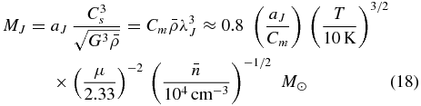
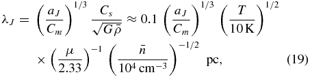
where μ is the mean molecular weight (=2.33 for cosmic composition), T the temperature of the gas, and aJ is a geometrical factor. For a uniform sphere, aJ = π5/2/6, and a top hat function in the real space, Cm = π/6, one gets the standard expression,  , with the Jeans mass being the mass enclosed in a sphere of diameter λJ. Because of the uncertainties in the smoothing filter (the window function), be they theoretical, numerical, or observational, and the shape and structure of the fluctuations, these masses and sizes inevitably retain some degree of uncertainty. If the star-forming clumps are filamentary, for instance, the mean thermal Jeans mass will differ by a factor of ∼0.6 from that of a sphere (Larson 2003). Given this uncertainty, we will simply adopt in the present paper for the Jeans length
  . Adopting a definition with a prefactor different from one simply translates into a uniform shift of the calculated IMF in mass and is thus degenerate with the value of the CMF-to-IMF (core-to-star) mass conversion efficiency (see below). All of these factors remain on the order of unity.
In both the Hennebelle–Chabrier and Hopkins theories, turbulence plays a key role in yielding the proper CMF and in determining the Salpeter-like slope at high masses (Chabrier & Hennebelle 2011), as confirmed by numerical simulations (Schmidt et al. 2010). A fundamental outcome of these theories is the concept of “turbulent Jeans mass, which is the mass at a given scale R that fulfills the aforementioned threshold condition for gravitational collapse in a turbulent density field. In the HC formalism, this mass reads

where the parameter  measures the importance of turbulence at the Jeans scale λJ, as opposed to the Mach number
  at the cloud scale Lc (see HC08):


where  denotes the Mach value at scale h and where we have made use of the scaling relations derived in Section 2.2. As explained in detail in Chabrier & Hennebelle (2011), the role of turbulence in defining such a characteristic mass should not be considered in a static (pressure-like) sense because turbulence has already dissipated by the time the prestellar core is formed, but rather in a statistical or dynamical sense, in selecting in the very initial field of density fluctuations those dense enough to not be dispersed by the flow before they have a chance to collapse. What matters in turbulence is thus the rms velocity rather than pressure. Equation (20) determines the transition between the thermally dominated (
 ) and the turbulence-dominated (
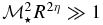 ) regimes, with the respective scaling relations for collapsing structures


where we have used Equation (5). We recall that n ∼ 3.8 denotes the three-dimensional velocity power spectrum index of turbulence. Note that for n = 4 (Burgers pressureless regime), i.e., η = 1/2, we recover exactly the scaling relations (8) for the rms velocity dispersion of star-forming clouds at constant pressure. It is worth mentioning that relation (24) yields for the bound prestellar cores M∝R1.8, consistent with the observational determination from Herschel, M∝Rβ, with β ∼ 1–2 (André et al. 2010; Könyves et al. 2010).
The transition limit between thermally dominated and turbulence-dominated regimes defines the equivalent of a sonic scale and a sonic mass:


The numerical coefficient in Equation (25) has been evaluated for n = 3.8, i.e., η = 0.4. These values are similar to those found in Hopkins (2012a). Equation (25) indicates that, in the HC formalism, the sonic length is entirely determined by the Jeans scale and the level of turbulence (Mach number) at this scale, illustrating the respective roles of gravity and turbulence in the mass–size relation of collapsing cores. Under typical MW conditions (V0 ≃ 0.8 km s−1, Cs ≃ 0.2 km s−1, then  ), this corresponds to Rs ∼ λJ, Ms ∼ MJ.
In the time-dependent version of the HC theory (Hennebelle & Chabrier 2011a, 2013), the number density mass spectrum of gravitationally bound cores reads
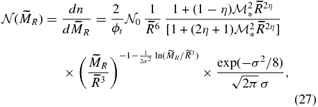
where  and ϕt is a dimensionless timescale factor that determines the typical time τ(R) within which a new density fluctuation of scale R is generated in the density field after the former one has collapsed, τ(R) = ϕtτff(R), where τff(R) denotes the fluctuation free-fall timescale. Theoretical estimates (Krumholz & McKee 2005; Hennebelle & Chabrier 2011a) and numerical simulations (Federrath & Klessen 2012) suggest ϕt ≈ 2. Strictly speaking, the mass spectrum in the HC theory entails a second member, which can also be calculated analytically (see Appendix B of HC08). However, as shown in HC08, this term becomes significant only when R ∼ Lc and will only impact the highest mass part of the IMF. For the sake of simplicity, this term will be dropped in the present calculations.
It should be noticed that the theory yields the mass spectrum of prestellar cores, i.e., the CMF, not the final IMF. As mentioned in Section 6, there is observational evidence that the latter strikingly resembles the former, with a uniform core-to-star mass conversion efficiency = M⋆/Mcore ∼ 0.3–0.7, due to the magneto-centrifugational outflows associated with the birth of the protostar (Matzner & McKee 2000). Because, as noted above, the ambiguity of the precise value of the geometrical and filtering parameters and thus of the Jeans length also translates into a uniform shift of the CMF, there is clearly a degeneracy between these two factors. This uncertainty, however, does not affect the general purpose and conclusions of the present study. Therefore, for the sake of simplicity, we will simply assume that the CMF (Equation (27)) represents the IMF. As seen from the above equations, the IMF only depends on the cloud's mean density
 for the normalization and the variance σ2 of the turbulence pdf for the shape (width and peak). As shown in Equation (16), this latter quantity only depends on the index n′ of the power spectrum of the log(density) of turbulence
 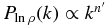 , with n′ ∼ n ∼ 3.8.
As demonstrated in HC13, the time dependence affects the static mass spectrum quantitatively through the normalization factor 1/ϕt but also qualitatively through the modification of the exponent,  , instead of
  in the static theory, which arises from the time dependence of the collapsing cores, proportional to
  (see HC13). This yields a steepening of the high-mass slope of the IMF.9 Physically speaking, this stems essentially from the fact that, during the collapse of the cloud, high-mass cores have time to fragment into smaller ones, an effect not accounted for in a static theory of the IMF. Time dependence also promotes the number of small cores because of their shorter free-fall timescale,
  , for a density fluctuation ρ(R). As examined below, this steepening of the IMF bears important consequences in very dense and turbulent environments.
As seen from Equation (27) (see also HC08, Section 5.4), the mass function entails a lognormal and a power-law contribution. This latter is dominant in the mass regime:

determined by the variance of the pdf, while the lognormal part produces an exponential cutoff outside these limits at small and large masses. Therefore, the stronger the turbulence (the higher the Mach), the larger the mass range covered by the power law part of the IMF and the smaller the mass at which it turns over a lognormal form. In the high-mass, turbulence-dominated regime (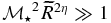 ), the power law part reads
  , with α = α1 + α2 and
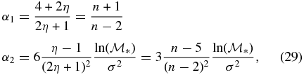
yielding α1 ≃ 2.66,  for n = 3.8.
For the usual MW molecular cloud conditions,  and
and  , the contribution from α2 is not negligible and decreases the slope to a Salpeter value, α ≃ 2.35. In contrast, for very dense (λJ ≪ Lc) and very turbulent (
 ) conditions, the second contribution has a weaker impact, so the slope is steeper than the canonical Salpeter one. It is interesting to examine under which conditions this second contribution provides only a negligible correction to the first one such that the slope remains close to α1. Clearly this occurs for very large Mach numbers, but it also implies a condition on
  and thus on the density. Using the definitions of
  and σ, a value |α2| ≲ 1% α1, for instance, yields as a rough condition (under the condition
  )
)

For T = 40 K, Lc = 100 pc,  , this corresponds to
  , for T = 60 K, Lc = 100 pc,
  , to
, to 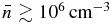 , and for T = 80 K, Lc = 100 pc,
  , to
, to  . Therefore, according to the present theory, in highly turbulent and very dense regions, the high-mass slope of the IMF is expected to be steeper than the Salpeter value, reaching up to a value of α = α1 ∼ 2.7. Not only has such a steepening of the IMF in massive ETGs been suggested by various studies (see Section 1), but also this maximum value for the high-mass slope is in remarkable agreement with the values inferred from recent spectroscopic observations (Spiniello et al. 2012) and dynamical determinations (Cappellari et al. 2012, 2013; Barnabè et al. 2013), which exclude slopes steeper than α ≈ 2.8 for ETGs with velocity dispersions in the range 200–335 km s−1.
In contrast, in low-density and weakly turbulent environments, the high-mass tail of the IMF can be shallower than the Salpeter value (see HC09, Figure 8). Such environments, however, barely form stars. Indeed, there have been claims in the literature that some dwarf galaxies, characterized by very low velocity dispersions (<10 km s−1) and SFRs four to five orders of magnitude smaller than in the MW, may have a shallower than Salpeter IMF slope (e.g., Geha et al. 2013). Although consistent with the general picture described by the HC theory, as just mentioned, these results must be taken with caution. The Geha et al. (2013) analysis relies on the study of a very narrow stellar mass range, namely 0.5–0.8 M☉, and drawing conclusions on the general behavior of the IMF, in particular based on a single power-law fit, is extremely uncertain. As clearly seen in the right-most panel of Figure 5 of that paper, narrow observed stellar mass ranges tend to predict shallower mass slopes, which might suggest a bias caused by limited statistics. This analysis must be confirmed over a more significant mass range before robust conclusions can be drawn.
The characteristic mass of the IMF, i.e., the most probable mass for collapse, is given by the peak of the IMF ( , which yields10
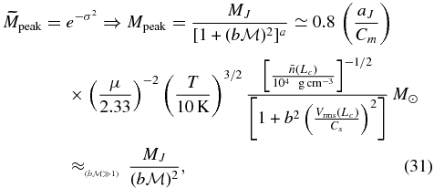
where b is the turbulence forcing parameter that enters Equation (17), ![$a=[1-(R/L_c)^{(n^\prime -3)}]$](https://content.cld.iop.org/journals/0004-637X/796/2/75/revision1/apj502960ieqn68.gif) (see Equation (16)), and T,
(see Equation (16)), and T,  , and Vrms denote the typical temperature, mean density, and large-scale velocity dispersion for a cloud of size Lc (mass Mc), as given by Equations (1), (2), and (12). The peak of the IMF thus also occurs at smaller masses the larger the typical Mach value of the cloud. It is interesting to examine the dependence of the peak of the IMF, Mpeak, on the cloud's mass, Mc, according to Equation (31). Combining this equation and Equations (1), (2), (18), and
  , one gets

where we have used η = 0.4 and where the two exponents for Lc and Mc correspond to ηd = 1 and 0.7, respectively. As noted in HC08 (their Section 7.1.4), the weak dependence of the peak mass of the IMF on the cloud's mass (a factor of 100 in mass yields a factor of ∼2 in Mpeak) certainly partly explains the observed universality of the IMF for similar density, temperature, and velocity dispersion conditions, i.e., similar T, d0, and V0.
Therefore, a major consequence of the concept of turbulent Jeans mass is that the characteristic scale or mass for fragmentation in a turbulent medium does not depend simply on the gas mean density and temperature, as in the standard Jeans mass concept of purely gravitational fragmentation, but also strongly on the Mach number. This again illustrates the respective roles of compressive turbulence motions, which generate the initial field of density fluctuations in the cloud, and gravity, which introduces a characteristic (Jeans) scale for gravitational instability. Physically speaking, comparing Equations (18) and (31), one can understand this result as the fact that the proper typical Jeans scale for fragmentation in a turbulent medium is no longer the one evaluated at the cloud's mean density but the one at the cloud's density compressed to higher values at all scales by the cascade of shock-dominated turbulence, ![$\bar{\rho }\times [1 +(b{\cal M})^2]^{a}$](https://content.cld.iop.org/journals/0004-637X/796/2/75/revision1/apj502960ieqn71.gif) . This differs drastically from star-formation theories invoking only gravitational fragmentation (e.g., Larson 2005), characterized only by the thermal Jeans mass. In the latter case,
. This differs drastically from star-formation theories invoking only gravitational fragmentation (e.g., Larson 2005), characterized only by the thermal Jeans mass. In the latter case,  , leading to a strong dependence of fragmentation on gas temperature. In that case, one would expect systematically bottom-light IMFs in warm (T > 10 K) environments. In the present theory, however, this temperature dependence is largely counterbalanced by the Mach dependence. As mentioned above, the reason for the “universality” of the IMF under MW-like conditions is the modest dispersion around the normalization values at 1 kpc, set up by the ones at the galactic scale, which are very similar for local galaxies, corresponding to a typical accretion rate ∼2 M☉ yr−1 from the IGM (Klessen & Hennebelle 2010).
As illustrated by the above relations, the HC theory of the IMF thus naturally predicts that the IMF of very dense and highly turbulent environments should have a characteristic (peak) mass shifted toward smaller masses compared with the standard MW Chabrier IMF and a high-mass slope that can be steeper than the Salpeter value. As mentioned above, this larger fraction of low-mass cores in such environments is a direct consequence of (1) the enhanced gas compression by highly turbulent motions, and (2) the shorter free-fall times for the collapsing overdense regions, increasing the relative fraction of small cores over massive ones, a process accounted for in the HC time-dependent formalism.
5. INITIAL MASS FUNCTIONS
5.1. Variations of the Initial Mass Function
Table 1 displays four typical star-forming cloud conditions characterized by different gas temperature, density, and velocity normalization values, d0, V0, as inferred in Section 3, within the expected range of cloud sizes. The characteristic virial parameter,  , measures the ratio of turbulence over gravitational energy within the clump. The case labeled “MW” is representative of typical MW conditions, with cloud sizes Lc ≃ 1–50 pc. Cases 1–3 should be representative of the conditions encountered in the high-redshift progenitors of massive ETGs and starburst environments, as discussed in Section 3, with enhanced gas temperatures, mean densities, and dispersion velocities, for cloud sizes Lc ≃ 1 to 100 pc. Figure 1 portrays the corresponding IMFs, calculated with Equation (27) with b = 0.5, the value inferred in simulations for high Mach numbers (Federrath 2013; Kritsuk et al. 2013). For each case, the two solid lines display the IMFs corresponding to the aforementioned bracketing cloud sizes. As mentioned earlier, in ULIRG-type galaxy mergers, the clouds form a nearly continuous medium rather than an ensemble of individual entities (Downes & Solomon 1998). For such a case of spatially close dense clumps, there is no need to sum up over a clump population because the HC theory naturally takes into account the clumpy structure of the gas, and the IMF for a given typical cloud size should be representative of the galaxy-wide IMF for a galaxy of similar typical scale height. In less dense environments, where clumps can be spatially well separated by diffuse gas, however, one must sum up over the clump population. This is illustrated by the long-dashed lines, which correspond to a global IMF integrated over a mass spectrum
  of molecular clumps, as given by Equation (16) of HC08. We recall that the mass spectrum
  obtained in the HC theory accurately recovers the one observed for CO clumps or infrared dark clouds in the MW,
  (e.g., Heithausen et al. 1998; Kramer et al. 1998; Peretto & Fuller 2010) (see HC08). This yields for the clump-integrated IMF

where  is the mass spectrum of self-gravitating cores (Equation (27)) for a clump of mass
  and volume Vc. The limits
  and
and  correspond to the minimum and maximum mass for these clumps according to the Larson relations (Equations (1)) for the clump sizes and density normalizations given in Table 1.
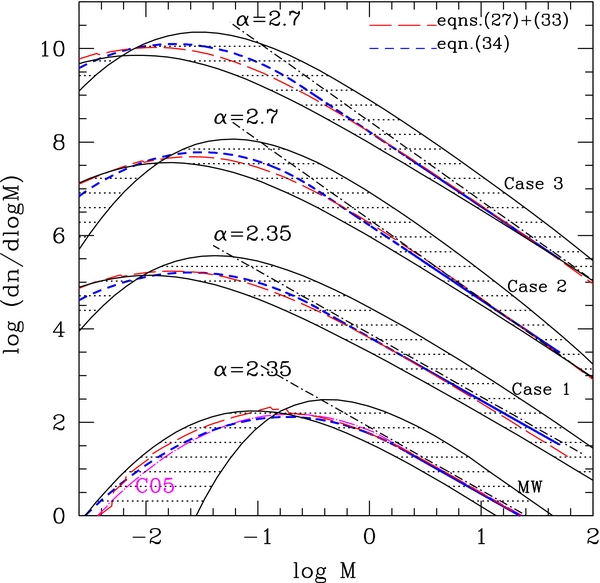
Figure 1. Initial mass function according to Equation (27) for conditions corresponding to the MW case and Cases 1, 2, and 3, respectively, from bottom to top (masses in M☉). In each case, the two solid curves correspond to single clumps of size L = 1 pc (right-most) and 50 pc (left-most), respectively, for the MW, and L = 1 and 100 pc for the other cases. The long-dashed (red) curves portray the integrated IMF for a clump mass distribution (Equation (33)), and the short-dashed (blue) curves correspond to the parameterized IMFs (Equation (34)). The dot–dashed lines correspond to the Chabrier (2005) object IMF (bottom, magenta, labeled C05), the Salpeter (1955) IMF (α = 2.35), and to power-law mass functions dn/dM∝M−2.7, the expected steepest slope according to Equation (29). For the sake of clarity, each group of curves for a given case has been shifted upward.
Download figure:
Standard image High-resolution imageTable 1. Star-forming Cloud Conditions for a Range of Cloud Sizes Lc, Characterized by Different Temperatures and Density and Velocity Dispersion Normalizations at 1 pc, d0, V0
| MW | Case 1 | Case 2 | Case 3 | |
|---|---|---|---|---|
| T (K) | 10 | 40 | 60 | 80 |
| d0 ( cm−3) | 3.5 × 10³ | 3.0 × 10⁵ | 1.0 × 10⁶ | 3.0 × 10⁶ |
| V0 (km s−1) | 0.8 | 5.0 | 5.0 | 8.0 |
| Cs (km s−1) | 0.19 | 0.38 | 0.46 | 0.53 |
| Lc (pc) | 1–50 | 1–100 | 1–100 | 1–100 |
 ( cm−3) ( cm−3) |
3.5 × 10³–2.2 × 10² | 3.0 × 10⁵–1.2 × 10⁴ | 1.0 × 10⁶–4.0 × 10⁴ | 3.0 × 10⁶–1.2 × 10⁵ |
| Mc ( M☉) | 1.0 × 10²–0.8 × 10⁶ | 8.9 × 10³–3.5 × 10⁸ | 3.0 × 10⁴–1.2 × 10⁹ |  –3.5 × 10⁹ –3.5 × 10⁹ |
| MJ ( M☉) | 0.7–3.5 | 0.7–3.8 | 0.8–3.8 | 0.7–3.4 |
| λJ (pc) | 0.2–0.8 | 0.04–0.2 | 0.03–0.15 | 0.02–0.1 |
 |
4–20 | 13–83 | 11–70 | 15–94 |
 |
1.3–2.2 | 2.2–4.2 | 1.5–2.9 | 1.8–3.4 |
| αvir | 1.2–0.2 | 0.5–0.05 | 0.2–0.02 | 0.15–0.02 |
Download table as: ASCIITypeset image
For the sake of simplicity and in order to focus on the very issue explored in the present paper, namely variations of the IMF under non-MW-like conditions, the present calculations have been conducted for the case of an isothermal gas for the respective temperatures given in Table 1. As shown in HC09, taking into account the thermodynamics of the gas will extend the IMF into the low-mass domain for an adiabatic index γ < 1. Given our lack of a precise knowledge of the dominant heating and cooling mechanisms in extreme starburst environments and given the expected large variety of conditions in such regions, it seems reasonable to stick for now to the simplest assumption. For the same reason, we do not explore the modification of the IMF due to binaries, so the IMFs correspond to unresolved stellar systems. The IMFs of unresolved systems and for individual objects are very similar in the stellar regime (Chabrier 2005). Notable differences start to emerge in the brown dwarf regime, unobservable in ETGs. Corrections due to binaries, although affecting to some level the IMFs displayed in Figure 1, should thus remain modest in the present context, certainly well within the uncertainties pertaining to the exact density, turbulence, and temperature conditions for extreme environments. Finally, the pdf of turbulence in the present calculations is supposed to obey a lognormal form, with the same value n′ = n for the respective indices of the log-density and velocity power spectra. Although, as mentioned earlier, these behaviors are verified in numerical simulations for moderate Mach values ( ), they certainly become more dubious for higher values (e.g., Kowal et al. 2007; Federrath & Klessen 2013). Again, the impact of the departure from these approximations on the results is likely to remain well within the range of uncertainties and expected variations characteristic of extreme star-forming conditions. We also recall that the HC theory does not depend on any specific pdf, although a lognormal form allows a fully analytical derivation.
The Chabrier (2005) IMF is shown for comparison in the figure, as well as the Salpeter IMF (dn/dln M∝M−(α − 1), with α = 2.35) and a power law IMF with α = 2.7. Even though the general behavior of the IMF remains the same for all conditions, with the combination of a power law at large masses and a lognormal form at smaller masses, large Mach values and high densities shift the peak toward smaller masses compared with the MW case, with the power law part extending eventually down to the hydrogen-burning limit, ∼0.1 M☉, in spite of the significantly larger gas temperatures. This reflects the general analysis carried out in the previous section. As mentioned earlier, in the standard Jeans gravitational theory for fragmentation, such high temperatures would predict the opposite behavior because the characteristic mass for fragmentation, namely the mean thermal Jeans mass, would be shifted toward higher masses. As seen in the figure, for Case 2 and more notably Case 3, which approach or fulfill the condition (30), the IMF can get steeper than the traditional Salpeter value over a significant mass range, reaching a slope value of α ∼ 2.7, as expected from our previous analysis.
As mentioned in Section 3.3, the temperature of the gas in the progenitors of ETGs and in starburst environments is rather uncertain, so it is interesting to examine the impact of such an uncertainty on the resulting IMF. This is illustrated in Figure 2, where we compare the IMFs obtained with Cases 2 and 3 under the same density conditions but with different temperatures, namely T = 80 K for Case 2 and T = 60 K for Case 3. As expected, a warmer medium implies a larger thermal Jeans mass and a lower Mach number (larger speed of sound), slightly shifting the characteristic mass of the IMF toward larger masses, as expected from Equation (31). The shift, however, remains relatively modest compared with the one induced by the Mach number dependence.
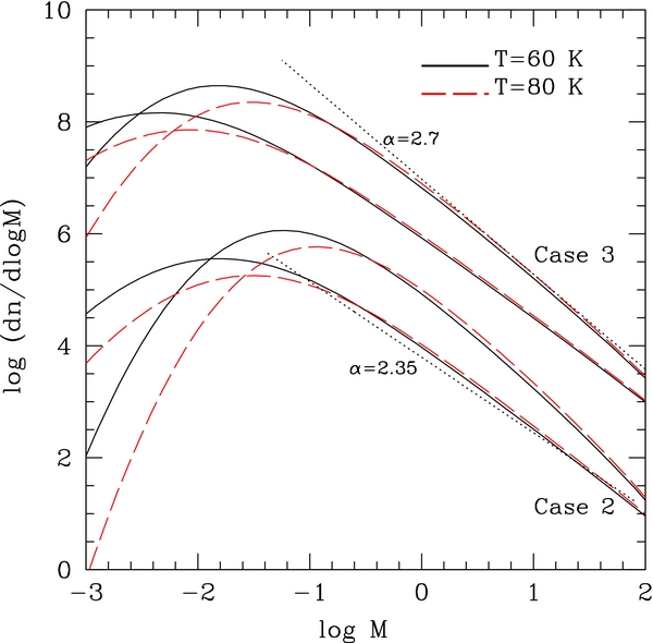
Figure 2. Initial mass function as in Figure 1 for Cases 2 (bottom) and 3 (top) for two cloud sizes, Lc = 1 pc (right curves) and Lc = 100 pc (left curves), for the same density conditions as given in Table 1 but different temperatures, T = 80 K and T = 60 K.
Download figure:
Standard image High-resolution imageThe case of globular clusters. An interesting issue can be raised at this stage concerning globular clusters (GCs). Indeed, although GCs are thought to have also formed under extreme conditions (high densities, large Mach numbers), their stellar mass function is not bottom heavy (see, e.g., Chabrier 2003, Figure 9). The formation of GCs, however, is still an unsettled issue (see, e.g., Renzini 2008). There is both photometric and spectroscopic observational evidence that GC formation occurred through a series of multiple stellar generations. Whether this happened in a short series of successive bursts or in a more continuous process is unclear, but the implication is star-formation episodes in an environment already inhabited by previous stellar populations. This mode of star formation differs from the case of GMCs devoid of preexisting stars, as examined in the present context. Furthermore, GCs have experienced dynamical evolution and tidal interactions, leading to a mass segregation of stars with time and space and yielding notably a deficiency of low-mass stars (Baumgardt & Makino 2003; Paust et al. 2010). Recovering the exact IMF from the observed present-day mass function in GCs requires dedicated dynamical evolution calculations, which will be highly valuable to explore.
5.2. Large Brown Dwarf Populations?
Looking at the bottom-heavy IMFs displayed in Figure 1, one may wonder whether the IMF extends to very low masses, suggesting the presence of a significantly larger brown dwarf population in these galaxies than in the MW, which has a star-to-brown dwarf ratio N⋆/NBD ∼ 4 (see Chabrier et al. 2014 for a recent review). The bottom of the mass function, however, might be truncated at higher masses than under MW-like conditions, precluding such a large brown dwarf population. Indeed, the IMF extends by definition down to the minimum mass for fragmentation, Mmin, defined as the density at which the balance between compressional heating and radiative cooling in a collapsing cloud, which ensures isothermality, breaks down. At this point, heating by compression of the gas is so effective against cooling that it stops the collapse, leading to the formation of a central adiabatic core. As shown by Masunaga & Inutsuka (1999), however, for a given mean opacity, the dependence of Mmin on the cloud temperature changes not only quantitatively but also qualitatively respectively below and above some temperature. For an opacity κ ∼ 0.01 cm2 g−1, which corresponds to a dust continuum opacity (the usually dominant coolant in the ISM) that is independent of the velocity structure of the cloud (in contrast to line cooling), this change in behavior occurs around T ∼ 30 K (Figure 3 of Masunaga & Inutsuka 1999). While Mmin decreases with increasing T below this value, it increases with T above it. The physical reason for this behavior is that, if the medium is warm enough, the radiative cooling rate is too large to be balanced by compressional heating, and thus the gas in the collapsing core becomes optically thick before isothermality breaks down, in contrast to what occurs in a much cooler medium. At this stage, cooling becomes ensured by radiative diffusion, which drastically reduces the radiative cooling rate ( , where
  is the gas optical depth). This increases by the same amount the rate at which the gravitational energy of the collapsing core is transported outward before being radiated away, then halting the collapse at larger Mmin. According to Masunaga & Inutsuka, in this regime Mmin depends on temperature as Mmin∝(T/10 K)(5 + 2ζ)/6, where ζ determines the temperature dependence of the opacity, κ∝κ0 × (T/10K)ζ and ζ ≃ 2 in this temperature regime (Bell & Lin 1994). This yields about a factor of ∼ times 10 increase of Mmin for T ∼ 40 K, and a factor of ∼ times 20 for T ∼ 70 K, yielding in the latter case Mmin ≈ 0.1 M☉ or about the hydrogen burning limit. Moreover, above the same temperature limit, Mmin is found to increase with opacity as Mmin∝κ1/3. Because the metallicity observed in ETGs today is slightly oversolar, with [α/Fe] ≃ 0.2–0.5 (Thomas et al. 2005), the opacity in these environments is expected to be larger than for MW GMCs, increasing further the Mmin. Finally, under such hot and dense environments, compressional heating of the gas becomes increasingly effective (
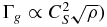 in heating up the cloud sufficiently against cooling. Therefore, given the expected larger gas temperatures, densities, and opacities in the progenitors of ETGs or in starburst environments, we expect the minimum mass for fragmentation to be substantially larger than under standard MW-like conditions, truncating the IMF at a mass limit closer to the hydrogen-burning limit.
Interestingly enough, recent observations combining gravitational lensing, stellar dynamics, and spectroscopic analysis of two massive early-type lens galaxies, yielding constraints on the total and stellar masses, respectively, suggest a Salpeter-like IMF over the entire stellar regime but with a low-mass limit ∼0.12 M☉ (Barnabè et al. 2013). If confirmed, these observations bring support to the above analysis.
5.3. Parameterization of the Initial Mass Function
For practical purposes, the IMFs given by Equation (27) for the various cases displayed in the figure can be parameterized under a Chabrier-like form, i.e., a combination of a lognormal and a power law, respectively, below and above a typical mass m0, the proper form of the IMF according to the present gravoturbulent picture of star formation. However, in order to ensure continuity of the derivative of the IMF, we slightly modify the original form according to the suggestion of van Dokkum (2008):

with m0 = ncmc. Continuity of the function and its derivative implies the condition σ2 = log nc/(xln 10) for the variance and 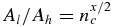 for the normalizing coefficients. Table 2 gives the values of m0, nc, σ, and x for the different cases examined in the present study, as well as the peak mass for the corresponding mass spectrum, dN/dM. These parameterized IMFs are illustrated by the short-dashed lines in Figure 1. A seen in the figure, the parameterized IMF labeled “MW” in Table 2 is very similar to the standard Chabrier (2005) IMF for resolved objects, characteristic of the MW environment. The number and mass integrals can easily be calculated analytically:
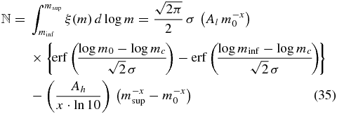
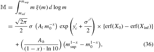
where  , σ′ = σ × ln 10 and
 ![$X_i=[y_i^\prime -(y^\prime _c+\sigma ^{\prime ^2})]/({\sqrt{2}}\,\sigma ^\prime)$](https://content.cld.iop.org/journals/0004-637X/796/2/75/revision1/apj502960ieqn91.gif) . These parameterizations will be useful in galaxy evolution calculations to explore the consequences of varying IMFs under nonstandard star-forming conditions such as the ones explored in the present study.
. These parameterizations will be useful in galaxy evolution calculations to explore the consequences of varying IMFs under nonstandard star-forming conditions such as the ones explored in the present study.
Table 2. Parameters Defining the IMFs in Equation (34), and the Corresponding Peak Mass (in dn/dM, see Equation (31)), for the Different Cases Under Study
| MW | Case 1 | Case 2 | Case 3 | |
|---|---|---|---|---|
| x | 1.35 | 1.35 | 1.6 | 1.6 |
| m0 ( M☉) | 2.0 | 0.35 | 0.35 | 0.25 |
| nc | 11.0 | 14.0 | 11.0 | 14.0 |
| σ | 0.579 | 0.607 | 0.531 | 0.558 |
| mc ( M☉) | 0.18 | 0.025 | 0.032 | 0.018 |
| Ah | 0.649 | 0.417 | 0.390 | 0.367 |
| Mpeak ( M☉) | 0.03 | 4 × 10⁻³ | 5 × 10⁻³ | 3 × 10⁻³ |
Note. The value of the normalization constant Ah corresponds to the mass integral equal to unity in Equation (36):  .
.
Download table as: ASCIITypeset image
6. STAR-FORMATION RATES
The SFRs obtained with these different IMFs are calculated as in Hennebelle & Chabrier (2011a, 2013):

where  is the (time-dependent) IMF of prestellar cores given by Equation (27), and Mcut is the largest unstable mass in the cloud, typically a fraction of the latter (see HC13). The parameter
 = M⋆/Mcore is the efficiency with which the mass within the collapsing prestellar core is converted into stars, i.e., the fraction of the prestellar core infalling gas effectively accreted by the nascent star. The other fraction is expelled by jets and outflows during the collapse (see Section 4). Then,
represents the local core-to-star formation efficiency. Calculations (e.g., Matzner & McKee 2000; Ciardi & Hennebelle 2010) as well as observations (e.g., André et al. 2010) suggest a value
≃ 0.3–0.7, yielding a factor (
/ϕt) ≈ 0.1–0.3. Note that SFRff is a dimensionless quantity, namely the SFR per cloud mean free-fall time
 , i.e., the fraction of cloud mass converted into stars per cloud mean free-fall time:
  (Krumholz & McKee 2005; Hennebelle & Chabrier 2011a, 2013; Federrath 2013). For star-forming galaxies, supposed to be marginally Toomre stable, Q ≈ 1, this timescale is approximately the disk orbital period (Krumholz & McKee 2005; Krumholz et al. 2012). The SFR at the global cloud scale, however, must also include the global efficiency, SFE, i.e., the typical fraction of star-forming (essentially molecular) gas effectively forming stars within clouds (i.e., within the galaxy, assuming all galactic molecular gas resides in clouds). Observations (Evans et al. 2009; Lada et al. 2010) as well as simulations (Federrath & Klessen 2013) suggest SFE ≈1%–6% within GMCs and a similar value for the galaxy-averaged star-formation efficiency (Kennicutt 1998; Swinbank et al. 2011). This yields a global SFR of

and thus a total volume and projected SFR densities, respectively:


where Σg is here the gas projected density evaluated for the area under consideration, be it a GMC or a galaxy. For a roughly homogeneous spherical cloud of size Lc,  , and for a galaxy of typical disk scale height h,
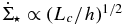
  . Clearly, the determinations of both the average free-fall time and gas density retain significant ambiguities (see, e.g., Krumholz et al. 2012; Evans et al. 2014). In particular, they both involve some scale over which they are averaged, assuming the gas distribution is uniform over this scale. As previously, we assume for simplicity that all of the galactic molecular gas resides in the GMCs, whose maximum size is the typical injection scale of turbulence, i.e., the galactic scale height (Section 2.2), so that Lc ∼ h (see, e.g., Krumholz & McKee 2005). Note that in the case where these two scales differ appreciably with Lc ≪ h, Equation (40) implies a dependence on the scale height as
  .
.
The traditional way to look at SFRs is to examine the relationship between  and Σg, as illustrated by the well-known Kennicutt–Schmidt relation
  . This is portrayed in Figure 3, as obtained from Equations (37), (38), and (40) for a global star-formation efficiency SFE = 1% for different cloud sizes (see figure caption), for the cloud characteristic conditions explored in the previous section11; we have used the average value
 /ϕt = 0.2. Observational results are displayed for comparison. Open symbols correspond to SFR determinations in disk local and high-z star-forming galactic regions, and solid symbols portray various data observed in starburst regions and high-z galaxies (see figure caption). As mentioned above, uncertainties both in
 and Σg determinations can easily translate into at least an order of magnitude or so uncertainty on these values. The dotted lines correspond to the theoretical calculations for MW conditions in Table 2 for SFE = 1%. As shown in HC11 and HC13, the HC theory adequately reproduces the observed SFRs in MW molecular clouds (see, e.g., Figure 7 of HC13).
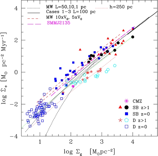
Figure 3. Global star-formation rates as a function of gas surface density for various conditions as obtained by Equation (37), assuming a global star-formation efficiency SFE = 1%. Thick (black) dotted lines: MW-like conditions in Table 1 for cloud sizes Lc = 1, 10, and 50 pc, from bottom to top. Thin (red) dotted line: MW-like condition for a cloud size Lc = 50 pc but a scale height h = 250 pc (see text). Superposed (barely distinguishable) black solid lines: density and velocity normalization conditions (d0, V0) corresponding to Cases 1–3 over a large density range for cloud size Lc = 100 pc. The corresponding Mach values,  , are given in Table 1. Long-dashed line: conditions characteristic of SMMJ2135. Short-dashed lines: MW-like density (d0) conditions but for normalization of the turbulent velocity amplitude at 1 pc, respectively, 5 times (5 × V0) (lower line) and 10 times (10 × V0) (upper line) the ones of the MW. For all of these calculations, we have adopted the average parameter value
 /ϕt = 0.2. Open symbols correspond to disk galaxies: Kennicutt (1998), blue squares; Daddi et al. (2010), red stars; Tacconi et al. (2010), cyan hexagons. Megenta asterisk: CMZ (Yusef-Zadeh et al. 2009). Solid symbols correspond to low-z and high-z starburst galaxies: Kennicutt (1998), blue squares; Bouché et al. (2007), red triangles; Genzel et al. (2010), solid black circles.
Download figure:
Standard image High-resolution imageSeveral conclusions can be drawn from the figure. First, as shown in HC11 and HC13, star formation still proceeds, although at small rates, in low-density environments, but mostly in large enough (Lc ≳ 10 pc) clouds. Indeed, only in such clouds is turbulence strong enough (according to Larson relations, see Table 1) to induce dense enough gravitationally unstable density fluctuations (see HC08). So there is no real “break“ or “threshold” in star formation but rather a continuous “bending” of the  versus Σg relation, which seems to be adequately reproduced by the theory. At higher density, such a scale dependence becomes weaker because the free-fall timescale of most density fluctuations becomes short enough for these regions to collapse before getting a chance to be wiped out by turbulent motions (see Chabrier & Hennebelle 2011). Second, the higher SFRs in starburst (SB) systems compared with disk (D) galaxies at the same gas surface density are well explained by the higher level of turbulence (higher Mach value) at all scales, as illustrated by Cases 1 to 3 but also by the short-dashed lines. These latter display our calculations for a density normalization d0 at 1 pc typical of the MW conditions but with a turbulent velocity amplitude normalization, V0, 5 times and 10 times larger than the standard value. Indeed, intense star-formation activity, typical of starburst conditions, implies a high rate of supernovae explosions, naturally increasing the level of turbulence at cloud scales. The (magenta) long-dashed line displays the results for conditions in star-forming clumps for the high-z massive galaxy SMMJ2135 (Swinbank et al. 2011). Star-formation densities in such environments are inferred to be about 15 ± 5 times higher than typically found locally (Genzel et al. 2010; Swinbank et al. 2010, 2012), in good agreement with our theoretical results. Third, the increasing SFRs with increasing redshift reflect not only the increasing level of turbulence but also the larger density normalization d0 (more compact structures), yielding shorter dynamical times.
These results suggest that at least part of the spread in the observed SFRs stems from variations in the general level of turbulence, illustrating the important role of the latter in star formation. Larger Mach values yield larger gas compression and thus higher SFRs. Indeed, both theory (HC11; HC13) and simulations (Padoan & Nordlund 2011; Federrath & Klessen 2012; Federrath 2013) show that turbulence overall enhances star-formation efficiency.
The calculations, however, overestimate the SFRs for high-redshift disk galaxies by up to an order of magnitude. Besides large uncertainties both in the theoretical parameters (, ϕt) and in the observational determinations, as mentioned above, one can examine possible explanations for this discrepancy. The first one would be a smaller fraction of molecular gas (
 ) in spirals than in starbursting systems, decreasing the global star-formation efficiency. Indeed, while the ISM in MW-like disks is essentially atomic, it is almost fully molecular in ULIRGs. A global efficiency SFE < 1%, however, is a rather low value. A second explanation is thicker disks in spirals compared with starbursts, with h > 100 pc, yielding a larger scale height and thus a lower projected SFR value. Scale heights in ULIRGS are indeed found to be substantially smaller than in the MW (Downes & Solomon 1998). As mentioned above, the SFR density depends on the scale height as
  . Therefore, using, e.g., a value of h = 250 pc would shift the MW dotted line obtained for Lc = 50 pc by a factor of log [(Lc/2h)1/2] = −0.5. This is illustrated by the thin red dotted line in the figure. In that case, the theoretical relation passes through the data at high density but lies at the very lower edge of the ones at low density. Therefore, the most apparent conclusion is that there seems to be a break in the slope of the
  versus Σg relation for disk galaxies near a gas surface density Σg ≈ 100 M☉ pc−2, with the slope becoming shallower above this value, in contrast to the starburst systems.
The green asterisk symbol in the figure portrays the SFR inferred for the CMZ for the appropriate gas surface density (Yusef-Zadeh et al. 2009; Kruijssen et al. 2014). As mentioned earlier, the velocity dispersions in this region are observed to be approximately ∼three to five times larger than for typical GMCs (e.g., Swinbank et al. 2011; Shetty et al. 2012; Kruijssen & Longmore 2013), resembling our typical Case 1 (see Table 1). The SFR relation corresponding to this latter case is illustrated by the lower part of the solid black line. For a gas surface density Σg = 120 M☉ pc−2, a cloud size Lc = 50 pc, and the gas scale height of the CMZ (Table 1 of Kruijssen et al. 2014), the predicted SFR surface density for Case 1 with our fiducial value SFE = 1% is  , about a factor two to three larger than the observational determinations,
  (Yusef-Zadeh et al. 2009; Kruijssen et al. 2014). Note, however, that the area actually filled with dense, star-forming gas is much smaller than the 500 pc globally averaged value used in the figure (see discussion in Kruijssen et al. 2014). Averaging gas and stars over the same area moves the data point to (log
  (S. Longmore, private communication).
These results clearly show the strong correlation between the SFR and the gas surface density, with an average slope consistent with the Kennicutt–Schmidt relation,  , as expected if
  . It has been suggested that, at high surface density, feedback, which is due, for example, to ionization, heating, or winds, overtakes turbulence as the main regulator of star formation (e.g., Renaud et al. 2012). Then, the characteristic timescale for star formation is no longer the free-fall time, but a given time after which the gas becomes available again for star formation. Because this timescale does not depend on density, this yields a linear slope
  . Given the large spread in the observed SFRs, however, it is not possible to favor one of the two relations, except possibly, as mentioned above, for the high-z disk galaxies. Feedback at a large (galactic) scale, however, certainly affects the global SFE, for instance by disrupting or photoionizing the clouds themselves, eventually shutting off star formation above some critical formation rate.
All in all, within the aforementioned range of expected global star-formation efficiencies, SFE ≈ 1%–6%, and local efficiencies, (/ϕt) ≈ 0.1–0.3, i.e., a 1.2 dex vertical spread, the present calculations well bracket all SFR determinations over five orders of magnitude in density, from local disk galaxies to high-z starburst systems. This strongly supports the idea of star formation resulting from a dominant, or more specifically two dominant universal mechanisms: turbulence, which generates the original field of density fluctuations, and gravity, which determines the dynamical time of these fluctuations, as described by the present general time-dependent gravoturbulent theory. The global efficiency, SFE, however, certainly depends upon the environmental conditions (or equivalently the initial conditions), notably the strength of turbulence at the injection scale and the mean density of the medium, which set up the density and velocity amplitude normalizations in Larson relations at the cloud scale.
It has been suggested (e.g., Krumholz et al. 2012, KDM) that plotting  as a function of Σg/τff instead of Σg provides a better representation of the SFR relation than the one displayed in Figure 3. This is illustrated in Figure 4, still with SFE = 1% in the calculations, where the observational values, including the free-fall time (more exactly dynamical time) determinations are the ones determined in KDM (as in Federrath 2013), keeping in mind that these values retain significant uncertainties. We have added to this figure the data for MW molecular clouds (Heiderman et al. 2010; Gutermuth et al. 2011). The spread in
  is still significant. As noted above and stressed in HC11 and HC13, the SFR not only depends upon density, but also strongly depends on the cloud's size or mass, in particular at low surface density. So strictly speaking there is no “universal“ star formation relationship between
  and Σg with a unique exponent, but rather different relations, depending on the cloud physical properties, with significant variations leading to a large dispersion, a point also supported by observational analysis (Shetty et al. 2013, 2014). As mentioned above, this scale dependence reflects the dominant role of large-scale turbulence as the main driver for star formation because the Mach number increases with Lc (Equation (2)). There is thus a degeneracy between the level of turbulence and the global star-formation efficiency, the two quantities being interconnected. Therefore, although the data are roughly consistent with an average value SFR ≈ 1% in Equation (40), i.e.,
  , as suggested by KDM, this global relationship must be taken with caution. Indeed, such a fixed efficiency does not capture the aforementioned dependence of star-formation efficiency on turbulence and thus on the cloud's scale (see, e.g., Evans et al. 2014).
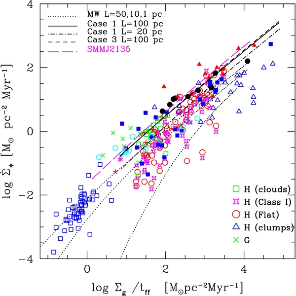
Figure 4. Global star-formation rates as a function of the gas surface density over a dynamical timescale (Equation (40)) for various cloud conditions, as displayed in the top left corner of the figure, for a global star-formation efficiency SFE = 1%. Data symbols are the same as in Figure 3, but we have added data for Milky Way molecular clouds from Heiderman et al. (2010, H) and Gutermuth et al. (2011, G).
Download figure:
Standard image High-resolution image7. MASS-TO-LIGHT RATIO
On the one hand, lensing observations constrain the total (maximum) mass of a galaxy within its Einstein radius. This comprises the total stellar mass, including stellar remnants, the ejected gas during stellar evolution, and the dark matter contribution. The stellar mass contribution, on the other hand, can be separated from the dark matter one with integral-field data using galaxy dynamical models (Cappellari et al. 2012, 2013). This eventually yields the stellar mass-to-light ratio, ϒ⋆ = (M/L)⋆. In ETGs, these ratios have been found to be ∼2× or more larger than those corresponding to a Chabrier IMF, typical of MW-like galaxies (Conroy & van Dokkum 2012a; Conroy et al., 2013; Cappellari et al. 2012, 2013; Tortora et al. 2013, 2014; Spiniello et al. 2012, 2014).
As mentioned earlier, star formation in the progenitors of massive ETGs must have taken place within a relatively short timescale. This is confirmed by the fact that the most massive galaxies, born in the highest density peaks of the primordial fluctuations, appear to be enhanced in α-elements (Section 1 and 3). This indicates that the duration of star formation decreases with increasing mass, having been shorter than ∼1 Gyr, the typical timescale for the onset of Type Ia SNe for the most massive galaxies. Hence, we can explore the stellar M/L ratios predicted by our formalism in these systems by using spectral evolution models for single stellar populations (SSPs). Figure 5 illustrates the evolution of ϒ⋆ as a function of age in various photometric bands obtained from SSP models (Bruzual & Charlot 2003) with the IMFs corresponding to the ones characterized in Table 2 and with a Salpeter IMF. Table 3 gives the corresponding values at an age of 10 Gyr, approximately the present age of observed ETGs. Changing the age of the stellar population in the SSP synthetic spectra anywhere in the range of ∼8 to 12 Gyr changes the M/L ratio by less than 20%. Note that these values represent only the stellar M/L ratios and do not include the brown dwarf contribution. Indeed, observationally, the stellar M/L ratios are determined essentially from the comparison of measured equivalent widths of given spectral lines (e.g., NaI, NaD, Ti02) characteristic of the low-mass star population with those derived from SSP synthetic models computed with different IMFs by fitting integrated spectra. They are thus only sensitive to the stellar population (note that the constraints on the stellar M/L from gravity-sensitive line strengths are degenerate with respect to the functional form chosen for the IMF; La Barbera et al. 2013). Moreover, as discussed in Section 5.2, the mass limit for star formation in extreme environments might be truncated at a significantly larger value than in the MW, precluding the existence of a large brown dwarf population. As seen in Table 3, the stellar M/L ratios in various passbands are in very good agreement with the ones inferred from various observations (e.g., Conroy & van Dokkum 2012b; Conroy et al. 2013). As mentioned earlier, the present calculations do not consider corrections to the IMFs due to stellar multiplicity. In order to estimate the impact of this correction upon the M/L ratios, we have calculated these values with the Chabrier (2005) IMF for unresolved systems and resolved objects, respectively. For all bands, the difference is less than 8%, significantly smaller than the differences between the values obtained with the various IMFs. This is not surprising because fragmentation of systems into multiple objects affects essentially the low-mass part of the IMF, and the effect remains modest in the stellar regime (see, e.g., Chabrier & Hennebelle 2010). Note that, in the cases of bottom-heavy IMFs, there is no need for a (significant) dark matter contribution, in agreement with recent observations of lens massive ETGs (Barnabè et al. 2013).
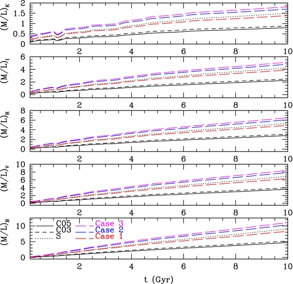
Figure 5. Stellar mass-to-light ratio, (M/L)⋆, as a function of age in various photometric bands obtained from SSP models using the IMFs corresponding to the Milky Way disk with the Chabrier 2005 IMF (solid line), the Chabrier 2003 IMF (short-dashed line), the Salpeter IMF (dotted line), and the IMFs corresponding to Cases 1 (red), 2 (blue), and 3 (magenta) (long-dashed lines going upward).
Download figure:
Standard image High-resolution imageTable 3. Mass-to-light Ratios ϒ⋆ in Various Bands at 10 Gyr Obtained for the Different IMFs Given in Table 2 and for a Salpeter IMF
| B | V | R | I | K | ϒ/ϒ⋆, MW | |
|---|---|---|---|---|---|---|
| MW | 4.7 | 3.6 | 2.8 | 2.3 | 0.8 | |
| Salpeter | 9.1 | 6.9 | 5.4 | 4.2 | 1.5 | ∼1.9 |
| Case 1 | 8.3 | 6.4 | 4.9 | 3.9 | 1.4 | ∼1.7 |
| Case 2 | 10.3 | 7.9 | 6.1 | 4.8 | 1.7 | ∼2.1–2.2 |
| Case 3 | 11.1 | 8.5 | 6.5 | 5.1 | 1.8 | ∼2.3 |
Notes. The last column gives the typical ratio ϒ⋆/ϒ⋆, MW. The MW values are calculated with a Chabrier (2005) IMF. Differences from a Chabrier (2003) IMF are ≲ 10%.
Download table as: ASCIITypeset image
At this stage, one should add a word of caution. As mentioned earlier, the metallicity inferred for ETGs is slightly oversolar, with [α/Fe] ≃ 0.2–0.5. One cannot rule out that the SSP models used to calculate M/L ratios are not correct for such metal-rich and α-enhanced stellar populations. One thus cannot completely exclude that the high inferred M/L values for such galaxies do not necessarily stem from a variation of the IMF but from a higher mass fraction in the form of stellar remnants. The integrated surface brightness of such a remnant population has been calculated by Chabrier (2004) and, although beyond present-day observational capabilities, might be detectable with the James Webb Space Telescope.
8. CONCLUSION
In this paper, we have shown that, under extreme conditions of very dense and turbulent gas, as encountered in starbursts or in the progenitors of massive ETGs, the characteristic (peak) mass of the IMF can extend to lower masses than under conditions typical of most spiral galaxies, in spite of the expected higher gas temperature. This is a direct consequence of the dominant role played by compressive turbulent motions in setting up the very initial field of density fluctuations that determine the initial conditions for star formation and the subsequent IMF. Indeed, in a gravoturbulent picture of star formation, the characteristic mass for fragmentation is not the mean thermal Jeans mass, as in the classical gravitational fragmentation scenario, but the turbulent Jeans mass, which strongly depends on the cloud's large-scale Mach number. At small scales, large-scale turbulence cascades into local shocks that drastically increase the local gas density, which in turn triggers the collapse of dense-enough regions into gravitationally bound prestellar core embryos. The consequences are a characteristic mass for the IMF in very dense and turbulent environments that shifts toward smaller masses compared with more quiescent or less dense conditions. According to the present theory, above some density the high-mass slope of the IMF in such environments can get steeper than the Salpeter value, reaching a limit of α ∼ 2.7, a consequence, in particular, of the time-dependence of the turbulence-induced fragmentation process, as incorporated in Hennebelle & Chabrier's (2011a, 2013) theory. The present results thus provide a theoretical foundation to observational indications that, while (less massive) spiral galaxies are consistent with a Chabrier IMF, more massive and dense ones, in particular massive ellipticals, require a Salpeter or even steeper IMF.
We provide simple estimates of the cloud typical properties, i.e., mean density d0 and velocity dispersion V0 normalizations at 1 pc, the relevant scale for the IMF, in terms of those at the galactic scale. The characteristic mass of the IMF is thus ultimately related to the prevailing conditions in the host galaxy, temperature, surface density, and velocity dispersion. As illustrated by Equation (32), for similar (T, d0, V0) conditions, the IMF is predicted to exhibit little variation, a consequence of the similar but opposite scaling dependence of the Jeans mass and rms velocity on a cloud's size. The theory then naturally explains the “universality” of the IMF for similar environments, i.e., similar values of T, d0, and V0.
We have parameterized IMFs representative of various extreme star-forming conditions to be used in stellar population calculations aimed at exploring IMF variations in various environments. We have also calculated the star-formation rates for these systems and confirmed that denser gas and larger turbulence significantly increase the SFR. SFRs in the progenitors of massive ETGs at high redshift should be orders of magnitude larger than at later epochs. We have also shown that the mass-to-light ratios calculated with the IMFs representative of the examined extreme conditions are consistent with the observationally inferred values. We speculate that in spite of an IMF characteristic mass extending to lower masses than for MW-like conditions, these systems do not necessarily contain a large brown dwarf population because for the corresponding temperatures the minimum mass for fragmentation should be significantly larger than for typical 10 K cloud conditions. Inferring the total dynamical mass, corrected for the dark matter contribution, and using one of the presently determined IMFs should enable us to confirm or not this suggestion.
The generic conclusion of the present calculations is that turbulence-induced star formation is indeed a universal mechanism and that star formation in massive, elliptical galaxies proceeded similarly as within disk and spiral galaxies but that gas density was much larger and turbulence was much more vigorous due mainly to intense accretion flows or merger events. The present fragmentation-induced turbulence theory for star formation naturally predicts that the IMF will become increasingly bottom heavy, and thus the mass-to-light ratio will increase in such environments, a consequence of the combination of high turbulence and density. We caution, however, that the evolution of the IMF does not necessarily correlate with the galaxy mass, i.e., the stellar velocity dispersion, but with its density and thus compactness, which is correlated with its mode of formation. We thus suggest that only massive galaxies having experienced rapid starburst episodes will have a bottom-heavy IMF, i.e., a large fraction of M dwarfs compared with “standards. These starburst events are a direct consequence of high accretion rates, which are due to merging events or intense gas flows, which not only increase the level of turbulence but also the density and thus the compactness of the galaxy. This might explain why the giant, low-density, elliptical ESO325-G004 seems to have an IMF compatible with the MW one, in spite of its large mass and velocity dispersion (>300 km s−1; Smith & Lucey 2013). A transition of the IMF might thus have occurred between massive galaxies that formed at high redshift by the merging of compact primodial structures dominated by strong gas flows and starbursts, followed by gas-poor merging, and spiral galaxies formed at lower redshift, where star formation proceeded essentially internally as a continuous, quiescent process. Because the progenitors of ETGs are the dominant galaxy population at high redshift, it might be interesting to revise accordingly the star-formation evolution in the universe using the various IMFs derived in the present study, although it is unclear what fraction of the total star formation has taken place in such extreme environments.
Footnotes
- 5
The Chabrier (2005) IMF adopts the same form as the Chabrier (2003) one but with a lower normalization at the hydrogen burning limit, determined from the updated nearby luminosity function released at that time (see Chabrier 2005 for details). These two IMFs differ essentially in the brown dwarf domain but yield similar M/L ratios in the stellar regime (see Section 7).
- 6
Clumps are usually defined as ∼parsec-size overdense regions in larger (∼10–100 pc) molecular clouds and are the very birth sites of star formation. They can be self-gravitating or not and are observed in CO absorption or dust emission. They are somehow a scale-downed version of GMCs, with slightly smaller sizes and larger mean densities. Their global properties are also similar to the ones of the clouds, so the term “clump” or “cloud” will be used indifferently to denominate the star-forming regions.
- 7
We recall that Vrms and V0 denote the 3D velocity dispersion (
 ) and that Σ0 denotes the surface density. Sometimes the projected density is used instead, which, for a sphere, introduces a factor of four because the projected area is A = π(L/2)2.
 - 8
As discussed below, the HC theory is essentially devoted to the formation of gravitationally bound prestellar cores and thus is truncated at scales larger than the cloud scale. Within this limit, the theory correctly accounts for the cloud-in-cloud problem in the original Press–Schechter formalism (see HC08; Hopkins 2012b).
- 9
- 10
For the sake of simplicity, we assume that the peak occurs in the purely thermal regime. A finite contribution from a turbulent velocity dispersion will shift the location toward slightly smaller masses.
- 11
As mentioned earlier, strictly speaking, the integral in Equation (37) in the Hennebelle–Chabrier theory involves two terms. The second term provides a truncation of the IMF at large scales, leading to slightly lower SFR values than the present ones. For the sake of simplicity, however, this term has been dropped in the present calculations (see HC11 and HC13 for details).


