ABSTRACT
The spectral absorption lines in early-type galaxies contain a wealth of information regarding the detailed abundance pattern, star formation history, and stellar initial mass function (IMF) of the underlying stellar population. Using our new population synthesis model that accounts for the effect of variable abundance ratios of 11 elements, we analyze very high quality absorption line spectra of 38 early-type galaxies and the nuclear bulge of M31. These data extend to 1 μm and they therefore include the IMF-sensitive spectral features Na i, Ca ii, and FeH at 0.82 μm, 0.86 μm, and 0.99 μm, respectively. The models fit the data well, with typical rms residuals ≲ 1%. Strong constraints on the IMF and therefore the stellar mass-to-light ratio, (M/L)stars, are derived for individual galaxies. We find that the IMF becomes increasingly bottom-heavy with increasing velocity dispersion and [Mg/Fe]. At the lowest dispersions and [Mg/Fe] values the derived IMF is consistent with the Milky Way (MW) IMF, while at the highest dispersions and [Mg/Fe] values the derived IMF contains more low-mass stars (is more bottom-heavy) than even a Salpeter IMF. Our best-fit (M/L)stars values do not exceed dynamically based M/L values. We also apply our models to stacked spectra of four metal-rich globular clusters in M31 and find an (M/L)stars that implies fewer low-mass stars than a MW IMF, again agreeing with dynamical constraints. We discuss other possible explanations for the observed trends and conclude that variation in the IMF is the simplest and most plausible.
1. INTRODUCTION
The stellar initial mass function (IMF) plays a central role in many areas of astrophysics. It sets the overall stellar mass scale of galaxies, determines the amount of energetic feedback following an episode of star formation (SF) via the ratio of high-to-low mass stars, governs the nucleosynthetic history of galaxies, and, more fundamentally, provides insight into the physics of SF.
Despite the central importance of the IMF, a comprehensive physical theory for its origin and variation with environment does not yet exist. It has been argued that the characteristic mass scale and shape of the IMF is set by the Jeans mass (e.g., Larson 1998, 2005), by feedback from protostars (Silk 1995; Adams & Fatuzzo 1996; Krumholz 2011), or by the distribution of densities in a supersonically turbulent interstellar medium (Padoan et al. 1997; Padoan & Nordlund 2002; Hennebelle & Chabrier 2008; Hopkins 2012a, 2012b).
Despite the variety of ideas, every theory predicts at least some variation in the IMF with physical properties. Remarkably, observations in our Galaxy of star-forming regions, open and globular clusters (GCs), and field stars have found little variation in the IMF (e.g., Scalo 1986; Kroupa 2001; Bastian et al. 2010; Kroupa et al. 2013). The observations are however complicated by a myriad of selection effects, biases, and correction factors. Observed luminosity functions must be corrected for binarity, stellar evolution, and, for GCs, dynamical evolution that preferentially ejects low-mass stars from the clusters. Moreover, direct constraints on the low-mass (M ≲ 0.5 M☉) IMF are limited to relatively mundane environments. Nonetheless, unambiguous evidence for IMF variation from direct star counts does not currently exist.
In nearby and distant galaxies, direct estimates of the IMF to ≈0.1 M☉ from star counts is currently impossible, and, except perhaps for a handful of Local Group galaxies, will remain impossible for the indefinite future. Less direct probes of the IMF are therefore required.
It was recognized in the 1960s that low-mass stars, though individually faint, can be detected in the integrated light of early-type galaxies (Spinrad 1962). Early attempts to exploit this fact to measure the IMF in early-type galaxies led to a variety of conflicting claims (Spinrad & Taylor 1971; Cohen 1978; Faber & French 1980; Carter et al. 1986; Hardy & Couture 1988; Delisle & Hardy 1992; Couture & Hardy 1993), owing largely to the inadequate quality of the data and models. Thanks largely to the increased quality of the stellar interior and atmospheric models and data in the intervening years, this technique is now capable of providing powerful constraints on the IMF (e.g., Cenarro et al. 2003).
In recent work we built a new population synthesis model that allows for arbitrary variation in the IMF, stellar age (for ages >3 Gyr), and the detailed abundance patterns of the stars (Conroy & van Dokkum 2012). In van Dokkum & Conroy (2010), we used a preliminary version of this new model to obtain constraints on the IMF in eight massive early-type galaxies in the Virgo and Coma clusters, finding evidence for an IMF in these galaxies that was much more bottom-heavy than the canonical Milky Way (MW) IMF (Kroupa 2001; Chabrier 2003). Following this work, in van Dokkum & Conroy (2011) we demonstrated that GCs in M31 with abundance patterns similar to the massive galaxies did not show evidence in their spectra for a bottom-heavy IMF, which was a critical test of the technique because such clusters are known not to have heavy IMFs from dynamical constraints (Strader et al. 2011). An increasingly bottom-heavy IMF with increasing galaxy mass has also been suggested by Spiniello et al. (2012) based on our models and data from the Sloan Digital Sky Survey.
Constraints on the IMF in early-type galaxies from kinematics and gravitational lensing also favor IMFs that become increasingly bottom-heavy toward higher galaxy masses (Grillo et al. 2008; Grillo & Gobat 2010; Treu et al. 2010; Auger et al. 2010; J. Thomas et al. 2011; Spiniello et al. 2012; Sonnenfeld et al. 2012; Cappellari et al. 2012). These techniques constrain the IMF by assuming that the stars and dark matter do not trace each other perfectly.4 This assumption becomes more plausible as the spatial distribution of the stars becomes less spherical (Cappellari et al. 2012).
Finally, constraints on the IMF from scaling relations and global models of galaxies and dark matter also favor an IMF that becomes increasingly bottom-heavy for more massive galaxies (Dutton et al. 2011, 2012a, 2012b).
This paper is the second in a series of papers aimed at measuring the IMF in early-type galaxies. In van Dokkum & Conroy (2012, hereafter Paper I) we present the sample, discuss data reduction techniques, and explore empirical trends in the absorption line spectra. In this paper we apply our stellar population synthesis (SPS) model to these data in order to simultaneously measure the stellar IMF, detailed abundance pattern, and mean stellar ages on a galaxy-by-galaxy basis.
We proceed as follows. In Section 2 we briefly summarize the observations, and in Section 3 we provide an overview of the model. The results are presented in Section 4, followed by a series of tests in Section 5, a discussion in Section 6, and a summary in Section 7.
2. DATA
Nearly all of the data analyzed in this paper have been obtained with the Low Resolution Imaging and Spectrometer (LRIS) on the Keck I telescope over the past three years. The early-type galaxy sample consists of a stacked spectrum of four massive galaxies in the Virgo cluster (originally from van Dokkum & Conroy 2010), 34 galaxies drawn from the SAURON sample of nearby early-type galaxies (Bacon et al. 2001; de Zeeuw et al. 2002), and the nuclear bulge of M31. For all galaxies except for the stacked Virgo spectrum and M31 the spectra are extracted within 1/8 of the effective radius, re. Details of the sample selection and data reduction can be found in Paper I.
We will also analyze spectra of four massive metal-rich GCs from M31. The red spectra for these objects were obtained with LRIS by us (van Dokkum & Conroy 2011), while the blue spectra were obtained with Hectospec by Nelson Caldwell, and kindly provided to us.
3. MODEL
We employ our new SPS model developed in Conroy & van Dokkum (2012, CvD12), with several minor extensions. The core of the model is based on two empirical stellar libraries: MILES (Sánchez-Blázquez et al. 2006) in the optical and IRTF (Cushing et al. 2005; Rayner et al. 2009) in the near-IR, at solar metallicity. Isochrones from the Dartmouth (Dotter et al. 2008), Padova (Marigo et al. 2008), and Lyon (Chabrier & Baraffe 1997; Baraffe et al. 1998) groups are combined to provide high-quality isochrones over the full stellar mass range appropriate for older stellar populations. SPS models are then constructed for ages ranging from 3 to 13.5 Gyr and for arbitrary IMFs by combining the isochrones with the empirical libraries. Constructing models with younger ages was not possible because the IRTF library does not currently include hot stars. In CvD12, we also computed a grid of fully synthetic stellar spectral libraries in order to model the variation of individual elemental abundances. In its present version, the model allows for variation in the elements C, N, Na, Mg, Si, Ca, Ti, Cr, Mn, and Fe, and O, Ne, S are varied in lockstep. We emphasize that the synthetic spectra are only used differentially with respect to the empirical libraries.5 The model makes predictions over the full optical and near-IR wavelength range of 0.36 μm < λ < 2.4 μm.
All models that feature simultaneous variation in multiple elements are constructed by assuming that the effect of each element on the spectrum is independent of the others. For example, a model with [Mg/Fe] = +0.2 and [N/Fe] = +0.2 is created by combining two models, one with only Mg variation and one with only N variation. This is an assumption in every model that includes variation in multiple abundance patterns (e.g., Thomas et al. 2003; Schiavon 2007). To our knowledge, this assumption has not been rigorously tested. We simply note it here as a possible systematic uncertainty in the modeling. This issue will be addressed in future work.
Moreover, we make the standard assumption that the response of the spectrum to variation in an element is linear in [e/Fe], where ‘e' stands for a generic element. In reality, the variation of spectral features with [e/Fe] is not linear in [e/Fe] when the range in [e/Fe] is large, especially for strong spectral features and for elements that play an important role in the atmospheric structure of stars. For most purposes this nonlinearity is not important, as the derived abundances do not vary significantly beyond the abundance range used to create the models (for example, our model spectra were computed with variations of ±0.3 dex for most elements). As we will see in later sections, this is not true for the derived [Na/Fe] abundances, which reach as high as 1 dex in our best-fit models. We have therefore computed new stellar spectral models with [Na/Fe] variation up to 0.9 dex and we use these new response functions in the present model. The use of these models, rather than linear extrapolations from the 0.3 dex models, results in a derived [Na/Fe] that is lower by ≈0.2 dex for the most extreme cases. Moreover, there is some evidence that non-LTE effects will result in stronger Na i lines compared to LTE models (Lind et al. 2011). To first order these effects should only change the derived [Na/Fe] abundance, but further work will be required to assess whether or not non-LTE effects can impact the derived IMF values as well.
Note that since abundance ratio variations are grafted onto empirical stellar spectra at approximately solar metallicity, the model is only applicable to systems with metallicities not too different from solar. The synthetic spectra allow us to create models with non-solar metallicities, but the extrapolation becomes less reliable as the metallicity deviates significantly from solar.
The model also allows for variation in the effective temperature, Teff, of the individual stars. This was implemented by computing new synthetic spectra with different Teff and then differentially modifying the empirical spectra. This parameter allows us to explore the effect of variation in the isochrones with metallicity. For example, a change in [α/Fe] by ±0.2 dex or [Fe/H] by ±0.1 dex results in a roughly 50 K change in the location of the isochrones near solar metallicity (e.g., Dotter et al. 2007, 2008). Most SPS models that consider variable abundance patterns do not include the abundance effects on the isochrones (e.g., D. Thomas et al. 2003, 2011; Graves & Schiavon 2008), with the exception of the models of Coelho et al. (2007) and Lee et al. (2009).
We emphasize that these models are the only ones currently available that follow the effect of individual elemental abundance variation on the full spectrum. To our knowledge, all other models that include variation in individual elemental abundances do so only on the effect of spectral indices, principally the Lick index system (e.g., Thomas et al. 2003; Schiavon et al. 2005; Lee et al. 2009).
In CvD12, we considered IMFs that were a single power law over the full mass range. In the present work we consider a three-component power law with separate indices, α1, α2, and α3, describing respectively the 0.1 M☉ < M < 0.5 M☉, 0.5 M☉ < M < 1.0 M☉, and 1.0 M☉ < M < 100 M☉ mass intervals. For reference, a Salpeter IMF has α1 = α2 = α3 = 2.3 and a Kroupa (2001) IMF has α1 = 1.3, α2 = 2.3, α3 = 2.3. Here we will fit for α1 and α2 and will fix α3 = 2.3. Stellar remnants are included in our M/L values according to a standard prescription (Conroy et al. 2009). A Kroupa (2001) IMF is adopted as our reference “MW” IMF.
We have also added several additional parameters meant to capture the addition of minority stellar populations. In addition to the age of the bulk population, we include a parameter to allow “frosting” (Trager et al. 2000) with a young population with an age of 3 Gyr (the youngest age in our model). We also include two parameters describing the contribution to the light from hot stars (whether they be young stars or hot horizontal branch stars). One of these parameters is the temperature of the star (ranging from 1–3 × 10⁴ K) and the second is the fraction of the total flux comprised of these stars. Finally, we allow for the addition of arbitrary amounts of M giant light (specifically an M7 giant). For our purposes we consider these as nuisance parameters, as our main goal is to measure the IMF from integrated light.
The fiducial model is characterized by 19 parameters: 11 for the abundance pattern, 1 for the age, 1 for Teff offsets, 2 for the IMF, 2 for the hot star component, 1 for the young component, and 1 for the fraction of additional M giant light. In addition to these 19 parameters, we also simultaneously fit for the velocity dispersion and redshift of each galaxy, bringing the total number of parameters to be fitted to 21. These parameters are summarized in Table 1.
Table 1. Model Parameters
| Parameter | Prior | Units | Notes |
|---|---|---|---|
| vz | (−1,000,10,000) | km s−1 | Recession velocity |
| σ | (20,400) | km s−1 | Velocity dispersion |
| [Fe/H] | (−0.4,0.4) | Iron abundance | |
| [O,Ne,S/Fe] | (−0.4,0.6) | Oxygen, neon, sulfur abundance | |
| [C/Fe] | (−0.4,0.4) | Carbon abundance | |
| [N/Fe] | (−0.4,0.8) | Nitrogen abundance | |
| [Na/Fe] | (−0.4,1.3) | Sodium abundance | |
| [Mg/Fe] | (−0.4,0.6) | Magnesium abundance | |
| [Si/Fe] | (−0.4,0.4) | Silicon abundance | |
| [Ca/Fe] | (−0.4,0.4) | Calcium abundance | |
| [Ti/Fe] | (−0.4,0.4) | Titanium abundance | |
| [Cr/Fe] | (−0.4,0.4) | Chromium abundance | |
| [Mn/Fe] | (−0.4,0.4) | Manganese abundance | |
| age | (4,15.0) | Gyr | Age of bulk population |
| log(fy) | (−5.0,−0.3) | Fraction of young (3 Gyr) stars | |
| α1 | (0.0,3.5) | IMF slope over 0.1 M☉ < M < 0.5 M☉ | |
| α2 | (0.0,3.5) | IMF slope over 0.5 M☉ < M < 1.0 M☉ | |
| α3 | 2.3 | IMF slope over 1.0 M☉ < M < 100 M☉ | |
| Δ(Teff) | (−50,50) | K | Temperature offset applied to all stars |
| log(M7III) | (−5.0,−0.3) | Fraction of additional M7III light | |
| log(fhot) | (−5.0,−0.3) | Fraction of additional hot stars | |
| Thot | (1,3) | 104 K | Temperature of additional hot stars |
Notes. The prior is flat within the range defined in the table and cuts off sharply outside of the prior range. The parameter α3 is fixed to the value 2.3.
Download table as: ASCIITypeset image
The native resolution of the model is not constant in velocity. In order to facilitate comparison to the data, we have broadened the models to a constant velocity dispersion of 100 km s−1. We note that the observed spectra have also been convolved to a resolution that is constant in velocity, with a dispersion of 100 km s−1 (see Paper I for details).
3.1. Fitting Procedure
We adopt a Markov Chain Monte Carlo (MCMC) fitting technique in order to efficiently explore the large parameter space of the model. In the MCMC algorithm, a step is taken in parameter space and this step is accepted if the new location has a lower χ2 compared to the previous location, and is accepted with probability  if the χ2 is higher than the previous location. Each step in the chain is recorded. After a sufficient number of steps, the likelihood surface produced by the chain will converge to the true underlying likelihood. Convergence is defined according to the prescription described in Dunkley et al. (2005). We have found that ∼105 steps are required in order to achieve convergence in all parameters. The “burn-in” region, where the chain is descending to the minimum of χ2, is removed before analyzing the chain, as is standard practice.
Priors on the model parameters must be specified in any MCMC algorithm to keep the chain from wandering into unphysical or unrealistic regions of parameter space. Our choice of priors on each parameter are specified in Table 1. Outside of the prior range, χ2 is penalized by a Gaussian with a width of σp = 0.01. The adopted priors have little impact on our results because the parameters are always well constrained within the prior range.
In the present work, we are most interested in the information contained in narrow spectral features. Therefore, we compute χ2 after dividing the model and data spectrum by a high-order polynomial. Operationally, we split the spectrum into four wavelength intervals 0.4 μm–0.46 μm, 0.46 μm–0.55 μm, 0.80 μm–0.89 μm, and 0.96 μm–1.02 μm, and divide each sub-region by a polynomial of degree n where n ≡ (λmax − λmin)/100 Å. Variation in n by ±2 induces changes to the spectrum at the ≲ 0.1% level.
The wavelength range 0.89–0.96 μm is not included because the sky absorption corrections are significant in that wavelength interval (see Paper I for details). While both the models and data extend to λ < 0.4 μm, the Ca ii H and K lines at 0.39 μm are not well modeled at the sub-percent level because these features form at very low densities in the stellar atmosphere. They are thus subject to non-LTE and three-dimensional effects, which are not included in the calculation of our synthetic spectra. As our goal is to model the observed spectra at the sub-percent level, we ignore the very blue end of the spectra. Nonetheless, the best-fit models, constrained at λ > 0.4 μm, do provide a good fit to the data at λ < 0.4 μm, with typical residuals at the several percent level. Examples of the quality of fit in the very blue are given in Figures 1 and 2, discussed below.
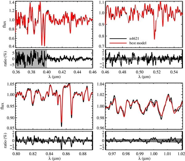
Figure 1. Comparison between the spectrum of NGC 4621 and the best-fit model. Within each plotted wavelength interval, continuum-normalized fluxes are shown in the top panel and the ratio between model and data is shown in the bottom panel. The gray shaded bands demarcate the noise limits of the data. The data at λ < 0.4 μm are not used in the fit; the gray shaded bands become very large in that wavelength range to highlight this fact. The light gray spectral regions are masked from the fit because of possible emission line contamination. NGC 4621 has one of the most bottom-heavy IMFs in our sample.
Download figure:
Standard image High-resolution image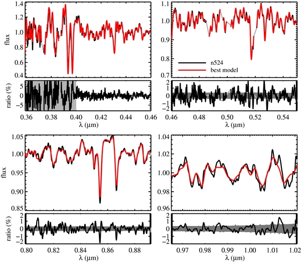
Figure 2. Comparison between the spectrum of NGC 524 and the best-fit model; see Figure 1 for details. NGC 524 has an inferred IMF similar to the MW.
Download figure:
Standard image High-resolution imageWe emphasize that the information contained in the broadband shape of the spectral energy distribution is not used in the fitting procedure. We choose this approach because it is very difficult to achieve accurate flux calibration over a large wavelength baseline at the percent level.
We mask the spectral regions surrounding the Hβ, [O iii], and [N i] emission lines and any spectral region contaminated by cosmic rays.
4. CONSTRAINTS ON THE IMF
In this section, we present constraints on the stellar IMF for a sample of early-type galaxies, the nuclear bulge of M31, and GCs. Other parameters derived from our SPS model, including detailed abundance patterns, will be presented in future work.
4.1. Early-type Galaxies
A typical fit to the continuum-normalized spectrum of an early-type galaxy is shown in Figures 1 and 2 for NGC 4621 and NGC 524, respectively. In these figures, we compare the observed spectra to the best-fit models. We also plot the ratio between the model and data and compare to the noise-to-signal ratio of the data. In the Appendix, we show the fits to the other 33 galaxies from Paper I.
In Table 2 we provide the mean signal-to-noise ratio (S/N) of the spectrum (averaged over the wavelength range used in the fit), the rms residual between the best-fit model and data, the minimum χ2/dof, the best-fit velocity dispersion, [Mg/Fe] and [Fe/H], the best-fit mass-to-light ratios in the r, I, and K bands allowing for IMF variation, and the best-fit mass-to-light ratio assuming a fixed MW (Kroupa 2001) IMF. All quantities are measured within an effective circular aperture of radius re/8 except for M31, which is within the central 4″ = 15 pc.
Table 2. Results from Stellar Population Synthesis Modeling
| Galaxy | 〈S/N〉 | rms (%) | χ2/dof | σ (km s−1) | [Mg/Fe] | [Fe/H] | M/Lr | M/LI | M/LK | (M/LK)MW |
|---|---|---|---|---|---|---|---|---|---|---|
| M 31 | 439 | 0.86 | 10.21 | 170 | 0.19 | 0.03 | 6.17 | 3.69 | 1.20 | 0.89 |
| NGC 474 | 219 | 0.76 | 2.13 | 178 | 0.17 | −0.05 | 2.98 | 1.88 | 0.69 | 0.58 |
| NGC 524 | 259 | 0.82 | 3.11 | 260 | 0.22 | −0.10 | 3.80 | 2.36 | 0.85 | 0.78 |
| NGC 821 | 266 | 0.69 | 2.55 | 216 | 0.20 | −0.05 | 3.71 | 2.30 | 0.81 | 0.68 |
| NGC 1023 | 440 | 0.63 | 6.14 | 217 | 0.18 | −0.01 | 5.26 | 3.20 | 1.04 | 0.68 |
| NGC 2549 | 371 | 0.76 | 6.28 | 157 | 0.12 | 0.07 | 1.92 | 1.22 | 0.42 | 0.63 |
| NGC 2685 | 189 | 0.95 | 2.27 | 96 | 0.13 | −0.03 | 1.80 | 1.16 | 0.41 | 0.50 |
| NGC 2695 | 221 | 0.75 | 2.11 | 210 | 0.25 | −0.09 | 5.81 | 3.56 | 1.28 | 0.76 |
| NGC 2699 | 180 | 0.81 | 1.72 | 154 | 0.15 | 0.03 | 3.80 | 2.39 | 0.87 | 0.66 |
| NGC 2768 | 239 | 0.89 | 2.97 | 222 | 0.19 | −0.09 | 2.98 | 1.85 | 0.64 | 0.67 |
| NGC 2974 | 260 | 0.75 | 2.90 | 247 | 0.20 | −0.06 | 5.22 | 3.21 | 1.16 | 0.80 |
| NGC 3377 | 352 | 0.77 | 5.88 | 140 | 0.19 | −0.06 | 2.52 | 1.60 | 0.57 | 0.49 |
| NGC 3379 | 431 | 0.65 | 5.96 | 225 | 0.24 | −0.08 | 5.58 | 3.40 | 1.12 | 0.70 |
| NGC 3384 | 432 | 0.71 | 7.74 | 168 | 0.13 | 0.05 | 2.08 | 1.30 | 0.41 | 0.65 |
| NGC 3414 | 264 | 0.84 | 3.89 | 243 | 0.23 | −0.09 | 4.92 | 3.00 | 1.04 | 0.79 |
| NGC 3608 | 271 | 0.76 | 3.25 | 194 | 0.22 | −0.10 | 4.31 | 2.67 | 0.93 | 0.70 |
| NGC 4262 | 227 | 0.68 | 1.78 | 214 | 0.27 | −0.10 | 6.96 | 4.21 | 1.45 | 0.78 |
| NGC 4270 | 132 | 0.80 | 0.88 | 150 | 0.08 | −0.01 | 2.38 | 1.54 | 0.60 | 0.59 |
| NGC 4278 | 286 | 1.05 | 6.23 | 273 | 0.32 | −0.25 | 8.68 | 5.08 | 1.61 | 0.87 |
| NGC 4382 | 328 | 0.66 | 4.18 | 184 | 0.11 | −0.02 | 1.05 | 0.69 | 0.25 | 0.40 |
| NGC 4458 | 167 | 0.97 | 2.08 | 116 | 0.26 | −0.19 | 3.75 | 2.37 | 0.94 | 0.56 |
| NGC 4459 | 269 | 0.71 | 2.70 | 186 | 0.12 | 0.00 | 1.94 | 1.26 | 0.46 | 0.57 |
| NGC 4473 | 270 | 0.58 | 2.03 | 194 | 0.20 | −0.01 | 4.56 | 2.82 | 1.01 | 0.75 |
| NGC 4486 | 244 | 0.82 | 3.17 | 385 | 0.33 | −0.16 | 9.82 | 5.66 | 1.71 | 0.90 |
| NGC 4546 | 286 | 0.73 | 3.04 | 233 | 0.24 | −0.03 | 7.16 | 4.30 | 1.40 | 0.78 |
| NGC 4552 | 329 | 0.68 | 3.90 | 271 | 0.26 | −0.00 | 8.41 | 4.97 | 1.55 | 0.76 |
| NGC 4564 | 238 | 0.76 | 2.52 | 175 | 0.22 | 0.04 | 5.14 | 3.10 | 0.96 | 0.73 |
| NGC 4570 | 229 | 0.67 | 1.82 | 194 | 0.20 | 0.02 | 7.19 | 4.27 | 1.37 | 0.79 |
| NGC 4621 | 343 | 0.68 | 4.30 | 232 | 0.25 | −0.02 | 7.20 | 4.34 | 1.39 | 0.71 |
| NGC 4660 | 240 | 0.64 | 1.79 | 212 | 0.24 | 0.00 | 4.50 | 2.74 | 0.89 | 0.73 |
| NGC 5308 | 167 | 0.60 | 0.82 | 241 | 0.24 | −0.07 | 4.76 | 2.93 | 1.03 | 0.73 |
| NGC 5813 | 204 | 0.86 | 2.33 | 233 | 0.28 | −0.12 | 4.62 | 2.85 | 1.04 | 0.76 |
| NGC 5838 | 231 | 0.62 | 1.46 | 290 | 0.21 | 0.01 | 5.86 | 3.57 | 1.21 | 0.73 |
| NGC 5845 | 166 | 0.57 | 0.70 | 263 | 0.22 | −0.00 | 5.38 | 3.29 | 1.09 | 0.74 |
| NGC 5846 | 192 | 0.87 | 1.95 | 246 | 0.26 | −0.07 | 7.23 | 4.34 | 1.46 | 0.82 |
Notes. The typical fractional error on M/L is 7% (statistical). Tests performed in Section 5.2 suggest that the systematic errors on M/L are not larger than 50%. The typical fractional error on (M/L)MW is 2% (statistical). The formal errors on [Mg/Fe] and [Fe/H] are <1%. All quantities are measured within an effective circular aperture of radius re/8 except for M31, which is within the central 4″ = 15 pc.
Download table as: ASCIITypeset image
In Figure 3 we show the covariance between several derived parameters and the mass-to-light ratio, M/L, for NGC 4621. The latter quantity is shown in units of the mass-to-light ratio assuming a MW IMF, (M/L)MW. Constraints on the IMF will be plotted in this way throughout the paper in order to isolate the effects of the IMF on M/L from the effects of age, [Z/H], etc. The most important point to take from this figure is the very weak or absence of a correlation between the IMF and other parameters. We have inspected a much greater cross-section of parameter space than what is shown in Figure 3 and find in general very little correlation between parameters, indicating that each parameter is well constrained by the data. It is also evident from this figure that the derived M/L is much larger than expected for a MW IMF. Indeed, NGC 4621 has one of the steepest IMFs in our sample (a Salpeter IMF is ≈60% heavier than a MW IMF, and so NGC 4621, with an M/L that is twice as heavy as a MW IMF, has an IMF even steeper than Salpeter).
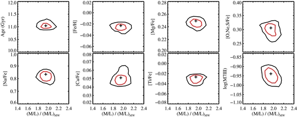
Figure 3. Covariance between various parameters and the normalization of the IMF. The latter is displayed as a ratio between the measured M/L and the M/L assuming a MW IMF. Results are shown for the fit to NGC 4621. The contours represent the 68% and 95% confidence limits (red and black lines, respectively). The symbols mark the median of the marginalized likelihoods. Note that there is weak or no correlation between the various parameters and the IMF, and that each parameter is very well constrained.
Download figure:
Standard image High-resolution imageNGC 4621 also has one of the highest [Na/Fe] values in our sample. The only sodium line being fitted is the Na i doublet at 0.82 μm; the NaD feature at 0.59 μm is not covered in the observed spectra. The constraint on [Na/Fe] is therefore coming from a combination of the feature at 0.82 μm and the fact that the sodium abundance has an indirect effect on the entire spectrum due to its influence on the free electron abundance in stellar atmospheres (see CvD12 for details). It is important to note that even when allowing the [Na/Fe] abundance to reach very high values, a bottom-heavy IMF is still favored for this particular galaxy. In other words, the very strong Na i feature is due both to high [Na/Fe] abundance and a preponderance of low-mass stars. A similar result was found by Spiniello et al. (2012) who analyzed the spectra of two higher redshift early-type galaxies. Spectra that cover the NaD feature will be very valuable for placing upper limits on the [Na/Fe] abundance. Of course, the NaD feature can only place an upper limit on the [Na/Fe] abundance because this feature may also be influenced by absorption from gas in the interstellar medium.
Before considering constraints on the IMF for the full sample, we first compare our best-fit [Fe/H] and [Mg/Fe] abundances to the [Fe/H] and [α/Fe] abundances6 derived for the same galaxies by Kuntschner et al. (2010, K10). The latter are based on the SPS model of Schiavon (2007). This comparison is shown in Figure 4. In K10 all of the α elements track each other (except for Ti), so [Mg/Fe] = [α/Fe] in that work. Note that the comparison is only approximate because K10 derive abundances within true circular apertures with radii equal to re/8, while we derive abundances within a slit of radius re/8 with a radial weighting meant to mimic a circular aperture (see Paper I). If the galaxies were perfectly smooth in the azimuthal direction, then the two approaches would yield identical spectra. However, it is clear from the two-dimensional stellar population maps in K10 that there is significant variation in the stellar populations at fixed radius. In any event, the iron abundances and α-enhancements generally agree to within ≲ 0.1 dex (the scatter between the two methods is 0.05 and 0.07 for [Mg/Fe] and [Fe/H], respectively), which is encouraging considering the different apertures and modeling techniques. It is also evident from Figure 4 that there is an anti-correlation between [Fe/H] and [Mg/Fe] such that the total range in metallicity, [Z/H], is only ≈0.2 dex.
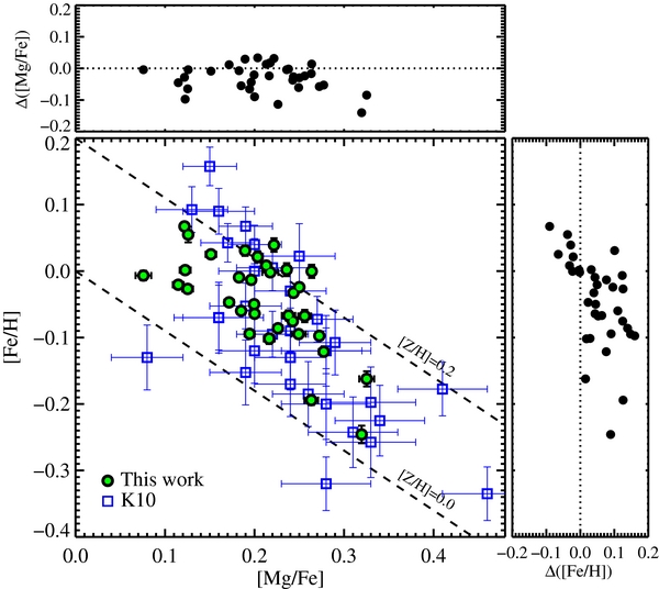
Figure 4. Comparison between [Fe/H] and [Mg/Fe] values derived in this work and in K10. The formal statistical errors on our measurements are often smaller than the symbol size. Dashed lines represent constant total metallicity, [Z/H]. The upper and left panels show differences between our and K10's measurements as a function of our values.
Download figure:
Standard image High-resolution imageThe principal result of this paper is shown in Figure 5. In this figure we show the K-band mass-to-light ratio, M/LK normalized to the mass-to-light ratio expected for a MW IMF. This quantity is directly related to the IMF and is plotted as a function of galaxy velocity dispersion, σ, and [Mg/Fe]. Error bars are marginalized 68% confidence limits. The most important conclusion to draw from this figure is that significant galaxy-to-galaxy variation in the IMF is inferred, ranging from IMFs slightly lighter than the MW to IMFs significantly heavier than the MW. In these units a Salpeter IMF has a value of ≈1.6, so there are galaxies that have inferred IMFs steeper even than Salpeter.
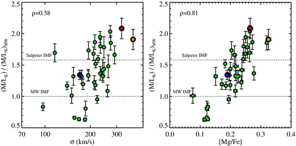
Figure 5. Best-fit M/LK in units of the best-fit M/LK for a MW IMF. This quantity is sensitive only to the IMF. Results are shown as a function of σ (left panel) and [Mg/Fe] (right panel). All galaxies would lie on the dotted line if the IMF was universal and of the MW form. The red symbol is the result for the stacked spectrum of four massive early-type galaxies from the Virgo cluster studied in van Dokkum & Conroy (2010), the orange symbol is M87, and the blue symbol is M31. The Spearman correlation coefficient, ρ, is included in the legend of each panel. The data therefore support a scenario wherein the IMF becomes steeper with increasing σ and/or [Mg/Fe].
Download figure:
Standard image High-resolution imageIn Figure 5, we also see clear evidence for correlations between the IMF and σ and between the IMF and [Mg/Fe]. The Spearman rank correlation coefficients, ρ, are 0.58 and 0.81, for the IMF correlation with σ and [Mg/Fe], respectively. [Mg/Fe] is an indicator of the SF timescale, and the fact that the IMF appears to correlate more strongly with this quantity than with σ suggests that the intensity of SF on kpc scales may play a key role in determining the shape of the IMF (see also Smith et al. 2012, who reach similar conclusions based on analyzing stacked spectra of galaxies in the Coma cluster). We return to this topic in Section 6.2.
Figure 6 shows the best-fit M/LK ratios as a function of the total metallicity, [Z/H], estimated as [Z/H] = [Fe/H]+0.94[Mg/Fe] (Thomas et al. 2003). The correlation here is much weaker than with either σ or [Mg/Fe] (ρ = 0.33), suggesting that total metallicity is not the fundamental variable driving IMF variation. The lack of correlation between [Z/H] and IMF is also an important diagnostic for any potential model systematic uncertainties that may correlate with metallicity, as we discuss further in Section 6.1.
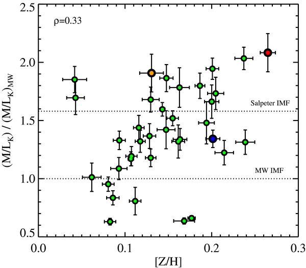
Figure 6. Best-fit IMF (plotted as in Figure 5) as a function of the best-fit total metallicity, [Z/H]. The Spearman correlation coefficient, ρ, is included in the legend. The correlation between IMF and [Z/H] is much weaker than between either σ or [Mg/Fe], suggesting that total metallicity is not the key variable driving IMF variation. This plot also implies that any model uncertainties that correlate with [Z/H] are unlikely to affect the qualitative IMF variation displayed in Figure 5.
Download figure:
Standard image High-resolution image4.1.1. Quality of Fit
Our constraints on the IMF are derived by marginalizing over 19 other parameters, including 11 parameters characterizing the detailed abundance pattern and 4 nuisance parameters meant to capture uncertain aspects of SPS modeling. Despite this high degree of flexibility, the error bars for most galaxies are inconsistent with a MW IMF.
Nonetheless, we might also ask how well fitted are the data by models in which the IMF is fixed to the MW value for all galaxies. We have thus re-fitted each galaxy in our sample with a model that is identical to the fiducial model except that the IMF is fixed to the MW value (specifically a Kroupa (2001) IMF). Inspection of the best-fit models confirms our expectation that the Wing–Ford band at 0.99 μm is a powerful IMF diagnostic when considered in conjunction with other spectral features (Conroy & van Dokkum 2012). In contrast, the Na i feature at 0.82 μm can be reasonably well fitted with a model without IMF variation but with higher [Na/Fe] abundance. The quality of the fit over the full spectral range for such models is, however, poorer (see below).
As an example of the quality of the fits, we show in Figure 7 a zoom-in on the Wing–Ford band for the two galaxies shown in Figures 1 and 2. In this figure the data are compared to two models, one in which the IMF is allowed to vary in the fit, and a second in which the IMF is fixed to the MW value. In the case of NGC 4621, where the best-fit IMF is significantly different from the MW IMF, we see that a fixed IMF model fails to capture the depth of the observed Wing–Ford band. This suggests that the Wing–Ford feature can be a strong discriminant between fixed and variable IMF models. In the case of NGC 524, there is essentially no difference between the predictions of the fixed and variable IMF models. This occurs because the best-fit variable IMF model returns a MW IMF for this galaxy. Nonetheless, both models predict a Wing–Ford band that is slightly too weak compared to the data for this galaxy. Formally the fits are acceptable, and we remind the reader that the data points are highly covariant owing to the velocity broadening of the spectrum.
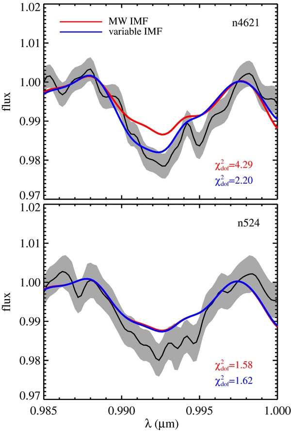
Figure 7. Zoom-in on the IMF-sensitive Wing–Ford band for NGC 4621 (top) and NGC 524 (bottom). These are the two galaxies shown in Figures 1 and 2. The observed spectrum (black line and gray band encompassing the 1σ errors) is compared to several best-fit models. The fiducial model, which fits the full wavelength range and includes parameters for the IMF (blue line), is compared to a model where the IMF is fixed to the MW value (red line). The χ2min is shown for each model fit, computed over the range 0.988 μm–0.997 μm. The spectrum of NGC 4621 is poorly fitted by a MW IMF, while the spectrum of NGC 524 is equally well fitted by a fixed or variable IMF model. Note that the best-fit models for NGC 524 are formally acceptable fits to the data around the Wing–Ford band, despite the appearance that the models slightly underpredict the feature strength.
Download figure:
Standard image High-resolution imageThe improvement in the quality of the fits when a variable IMF model is considered can be quantified by the difference in the minimum of χ2. Figure 8 shows Δ(χ2) between models that do and do not allow for variation in the IMF as a function of the difference in the best-fit M/L between the two models. The latter quantity is in units of the uncertainty in M/L. Selected galaxies are labeled in the figure. There is a clear trend in the sense that galaxies with mass-to-light ratios that deviate strongly from what is expected for a MW IMF have large Δ(χ2). This of course is not surprising, as it is precisely the χ2 value that the fitting routine uses to determine the best-fit M/L ratios.
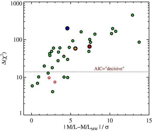
Figure 8. Difference in the minimum of χ2 between models with and without variation in the IMF, as a function of the difference in best-fit M/LK in units of the uncertainty. Symbol colors are as in Figure 5. The two open symbols have Δ(χ2) < 0 and so for these galaxies we plot |Δ(χ2)|. The model with IMF variation has two additional degrees of freedom compared to the fixed IMF model. In the context of the AIC, the variable IMF model is ‘decisively preferred for Δ(χ2) > 14; see the text for details.
Download figure:
Standard image High-resolution imageQuantifying the preference of one model over another is notoriously complex (see Liddle 2007 for a brief review). Among the most popular metrics are the Akaike and Bayesian information criteria (the AIC and BIC, respectively; Akaike 1974; Scwarz 1978). The former is defined as AIC≡ χ2 + 2k where k is the number of free parameters. The AIC attempts to balance a change in χ2 against increased model complexity. In our case the two models under consideration differ by two parameters, and so an equivalence in AIC would correspond to Δ(χ2) = 4. According to Jeffreys' scale, Δ(AIC) > 5 is judged as “strong” evidence for one model over another, while Δ(AIC) > 10 is judged as “decisive” (Liddle 2007). We can therefore associate Δ(χ2) > 14 as a threshold for decisive preference for the model with IMF variation over the model without IMF variation. This threshold is included in Figure 8. Note that every galaxy with >3σ evidence for an IMF different from that of the MW has Δ(χ2) > 14, indicating that, in the context of our model, the variable IMF model is very strongly (decisively) preferred. We have not considered the BIC herein because it depends on the number of data points and assumes that the data points are independent. This condition is clearly violated in our case because the velocity dispersion of each galaxy is larger than the wavelength sampling; adjacent data points are therefore highly correlated.
It is apparent that the observed CaT feature is not very well fitted by the models in Figures 1 and 2, especially in the cores of the lines. This issue is explored further in Figure 9. In the left panels we show residuals between the best-fit model and data around the CaT feature for all 35 galaxies, split according to their M/L ratio. Also included is the mean residual for the entire sample (red lines) and the mean residuals within each panel. Comparison of the green and red lines in these panels suggests that the CaT feature is poorly fitted for all galaxies, and the quality of the fit does not vary much with M/L. In other words, there appears to be an overall offset between the models and the data, independent of the best-fit IMF. Recall that the [Ca/Fe] abundance is included in the model fits, and is well constrained by the Ca i feature at 0.4227 μm. The offset between the models and data is therefore unlikely to be a calcium abundance effect.
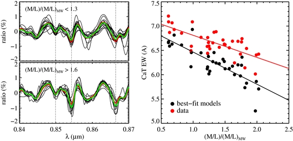
Figure 9. Comparison of models and data around the CaT feature. Left panel: residuals between the best-fit model and data for galaxies split according to their best-fit IMF (light IMFs in the top panel, heavy IMFs in the bottom panel). The green lines are the mean residuals within each panel, and the red line is the mean residual for the entire sample. Dotted lines mark the location of the CaT features. Right panel: comparison of the CaT EW between the best-fit models and the data as a function of the best-fit IMF. Solid lines are a linear fit to the trends. Note that while the best-fit models are offset low compared to the data, the trend of CaT strength with the inferred IMF is similar between the models and the data. These panels suggest that there is an overall offset in the predicted strength of the CaT feature in the current version of our models.
Download figure:
Standard image High-resolution imageThe tension between the observed and modeled CaT is displayed in another way in the right panel of Figure 9. Here we show the equivalent width (EW) of the CaT feature (see Conroy & van Dokkum 2012 for the definition of this index) for both the models and the data as a function of the best-fit M/L ratio. The overall trend of decreasing CaT strength with increasing M/L ratio is expected because the CaT is a giant-sensitive feature. The offset between the models and data is also apparent, and the offset is approximately constant with M/L. The origin of this offset is unclear. It may be due to the fact that the CaT absorption lines form at very low Rosseland optical depths, and so the model becomes sensitive to the treatment of the tenuous outer atmospheres of model giants. It may also reflect an underlying error in the construction of the base set of empirical models onto which the synthetic spectra are grafted. Regardless of the origin, the most important point is that the offset is almost completely independent of M/L, and implies that this tension between the model and data is unlikely to be driving the qualitative variation in the IMF that we observe.
4.2. The Nuclear Bulge of M31
The form of the IMF in the nuclear bulge of M31 was the subject of intense debate in the 1970s and 1980s. Spinrad & Taylor (1971) observed the Na i 0.82 μm feature and concluded that the bulge was dwarf-dominated ((M/L)stars = 44). A large number of subsequent observations have led to conflicting results (e.g., Oconnell 1976; Whitford 1977; Frogel et al. 1978; Cohen 1978; Faber & French 1980; Carter et al. 1986; Delisle & Hardy 1992). There is broad agreement that the Na i feature is quite strong, especially in the nuclear region (the inner 2″–4″). The debate centered on whether this enhancement is due primarily to an increase in the dwarf star contribution or an increase in the [Na/Fe] abundance. If interpreted as the former, the implied mass-to-light ratio would be M/LB ≈ 28 (Faber & French 1980), which would be in strong conflict with dynamical constraints (Saglia et al. 2010).
In light of the controversial history of the nuclear bulge of M31 we decided to include M31 in our analysis. The LRIS spectrum of M31 was extracted within a radius of 4″, which corresponds to the central 15 pc of M31. We fit our SPS model to this spectrum in a manner identical to the early-type galaxy data. The resulting best-fit M/LK is shown as a blue symbol in Figure 5. We derive a mass-to-light ratio that is in between a MW IMF and a Salpeter IMF, and is highly inconsistent with dwarf-rich (bottom-heavy) IMFs. As will be discussed in Section 5.1, our derived mass-to-light ratio for M31 agrees well with dynamical constraints (Saglia et al. 2010).
The nuclear spectrum shows an abundance pattern typical of the early-type galaxy sample. It is α-enhanced in all the α elements except for Ca and Ti, and also enhanced in N and C. The derived sodium abundance is however one of the highest of the sample, at [Na/Fe] ≈ 1.0. More detailed models and coverage of the NaD spectral feature will shed further light on the sodium abundance in M31 and other galaxies. Removal of the Na i feature results in a change in M/LK of −50%, while removal of both the Na i and CaT features results in a change in M/LK of +50%. These changes are typical of the systematic uncertainties in our present modeling technique (see Section 5.2 for details).
The basic result from this section is that the nuclear region of M31 is entirely consistent with a normal IMF. We can certainly rule out extreme mass-to-light ratios, such as those suggested by Faber & French (1980) based on data obtained within a slightly larger aperture (2″ × 4″ compared to an 8″ circular diameter herein). We derive much lower M/L ratios compared to Faber & French in part because we allow for large [Na/Fe] variation (reaching nearly 1 dex for the nuclear spectrum of M31), and in part because the FeH feature places a strong upper limit on the allowed M/L values.
4.3. Metal-rich Globular Clusters in M31
We now turn to constraints on M/L for four metal-rich GCs in M31. These clusters were selected to be metal-rich, α-enhanced, and old (Caldwell et al. 2011). They have stellar masses in the range 5.5 < log M/M☉ < 6.1, based on dynamical constraints, and long relaxation times (Strader et al. 2011). One of the most intriguing facts of these clusters is that their K-band mass-to-light ratios are a factor of ∼2 lighter than expected for a MW IMF (Strader et al. 2011). GCs are simpler than galaxies in the sense that the stars within them are approximately coeval, and they are known to contain little or no dark matter (Conroy et al. 2011, and references therein). Comparison between dynamical and stellar population-based constraints on M/L is therefore straightforward.
We have fitted the stacked spectrum of these four clusters with our model. The resulting best-fit K-band mass-to-light ratio is shown in Figure 10, plotted versus the best-fit [Mg/Fe] abundance. We also include our sample of early-type galaxies that have ages >10 Gyr.
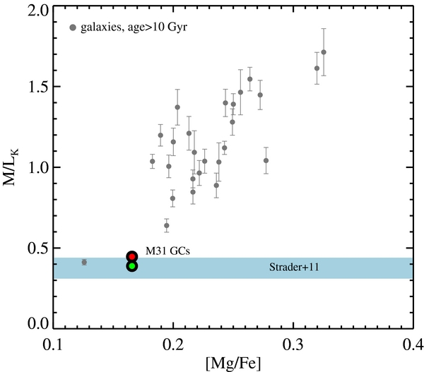
Figure 10. M/LK vs. [Mg/Fe] for the early-type galaxies analyzed in the present work (gray symbols) and for the stacked spectrum of four metal-rich globular clusters in M31 (red symbol; statistical error bars are smaller than the symbol size). We also compute and include in the figure the mass-to-light ratio computed without black hole and neutron star stellar remnants (green symbol). The dynamically based M/LK for the four M31 clusters is shown as a solid band (Strader et al. 2011). The M/LK for a 13 Gyr, solar metallicity MW IMF model is 0.9, implying that these globular clusters are lighter in mass than expected for a MW IMF, and consistent with dynamical constraints.
Download figure:
Standard image High-resolution imageThe standard model M/LK ratio, which includes a contribution from stellar remnants, is shown as a red symbol. We have also computed a mass-to-light ratio without inclusion of black hole and neutron star stellar remnants (green symbol). A paucity of remnants in GCs may arise because the shallow potential well of the GCs permits the escape of massive remnants when the progenitor star explodes. In any event, the effect of black holes and neutron stars on the mass-to-light ratio is small.
Dynamical mass-to-light ratios have been computed for these clusters by Strader et al. (2011); the full range spanned by these four clusters is shown as a band in Figure 10. For reference, a 13 Gyr, solar metallicity MW IMF model has M/LK = 0.9.
Both the stellar population-based and dynamically based mass-to-light ratios point toward a bottom-light IMF in these GCs. This broad agreement between two completely independent techniques is very encouraging, and lends support to our model results.
5. TESTS
In this section, we discuss several tests of our principle result that the IMF is not universal. We confront our best-fit models with dynamical constraints in Section 5.1 and we discuss several possible systematics in the model in Section 5.2.
5.1. Comparison to Dynamical Masses
In this section, we compare mass-to-light ratios estimated from our models to dynamical estimates. For the 34 galaxies drawn from the SAURON survey, dynamical mass-to-light ratios are based on Jeans axisymmetric modeling of the two-dimensional velocity field (Scott et al. 2009). For these galaxies the dynamical estimates are quoted within re. We have adopted a typical uncertainty on the dynamical M/L values of 6% following Cappellari et al. (2006).
The comparison between our stellar population-based mass-to-light ratio, M/LSPS, and the dynamically based M/Ldyn is shown in Figure 11. Mass-to-light ratios are quoted in the I band in order to provide a direct comparison with results from the SAURON survey (Scott et al. 2009). Note that the SPS- and dynamically based mass-to-light ratios are obtained within different physical apertures (re/8 for the former and re for the latter).
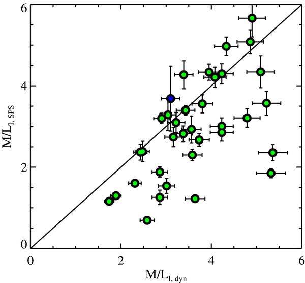
Figure 11. Comparison between SPS-based and dynamically based M/LI. Note that the SPS-based mass-to-light ratios never violate the dynamical constraints. M31 is shown separately (blue symbol) because the dynamical constraints on M/L come from a different source and technique than the rest of the sample. The M/LI, SPS ratio for a MW and a Salpeter IMF is 2.2 and 3.4, respectively, assuming an age of 13 Gyr and solar metallicity.
Download figure:
Standard image High-resolution imageSaglia et al. (2010) have estimated the dynamical mass-to-light ratio for M31 in the R band based on long-slit data. We have assumed (M/LR)/(M/LI)=1.3, appropriate for a 13 Gyr single-age population with solar metallicity, in order to translate their value into M/LI. Saglia et al. provide M/LR as a function of radius; we adopt a dynamical mass-to-light ratio within 4″ for comparison to our SPS-based value.
The SPS-based M/L values are always less than or equal to the dynamical M/L values within the 2σ errors, which is remarkable given the small size of the SPS-based errors. Even in cases where we infer bottom-heavy IMFs, the derived M/L values do not exceed the dynamical constraints. There are galaxies for which the SPS-based M/L ratios are less than the dynamically based ones. In these cases there is room for additional, non-stellar mass (i.e., dark matter).
5.2. Systematics
In this section we explore several variations to our fiducial model. The variations are of two types: changes to the spectral range included in the fit, and changes to the properties of the stellar population model. We consider the effect of these variations on the derived M/LK ratios.
We begin by considering variation in the spectral range included in the fits. In the top panels of Figure 12, we consider the effect on M/LK of removing one or more classic IMF-sensitive spectral features. In the left panel, we remove the Na i spectral region (0.81 μm–0.83 μm). In the middle panel, we remove both the Na i and CaT features (0.81 μm–0.83 μm and 0.845 μm–0.87 μm). In this case, the Wing–Ford band is the only classic IMF-sensitive feature included in the fit. In the right panel we remove from the fit all information beyond λ > 0.96 μm, which includes the Wing–Ford band.
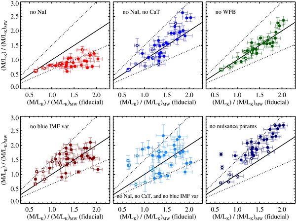
Figure 12. Exploration of systematic effects on the derived mass-to-light ratios. In each panel, the M/LK is plotted in units of (M/LK)MW (as in previous figures). Dashed lines indicate a slope change of ±50%. The open symbols in each panel indicate galaxies with ages younger than 10 Gyr. The upper panels highlight the effect of removing one or more spectral regions from the fit. In the left panel the Na i feature is removed, in the middle panel both the Na i and CaT features are removed, and in the right panel the Wing–Ford band spectral region is removed. Neglecting certain IMF-sensitive features affects the overall normalization of the M/LK values at the ≈50% level, but relative trends are robust. The lower panels highlight other model permutations. In the left panel, we turn off the spectral variation due to the IMF in the blue spectral region (λ < 0.8 μm), in the middle panel we turn off blue IMF variation and remove Na i and CaT from the fits, and in the right panel the three nuisance parameters are not included in the fit. In the middle panel, the only constraints on the IMF are coming from the Wing–Ford band spectral region. These tests suggest that the absolute M/LK ratios carry systematic uncertainties at the ≲ 50% level, and that the Wing–Ford band alone is likely not sufficient to place strong constraints on the IMF over the range of IMFs probed.
Download figure:
Standard image High-resolution imageQualitatively, we recover the same trends no matter which set of IMF-sensitive features is used. In particular, in all cases we find evidence for IMF variation. This provides strong confirmation that our basic result is not influenced by a single spectroscopic feature. There are however noticeable offsets between the various permutations, especially in the upper left panel of Figure 12. This means that in detail the various IMF-sensitive features are favoring different values of M/LK, which in turn suggests that there are residual systematics in the modeling. One possible explanation lies in the fact that these features are each most sensitive to a different range of stellar masses (see CvD12 for details). The data may be demanding an IMF that is more complicated than the broken power law that we adopt. These issues will be explored in future work.
We have also considered a model where the effect of the IMF on the spectrum is limited to the red (λ > 0.8 μm). In this model, the blue spectrum is completely insensitive to IMF variation. Our goal here is to assess the extent to which the IMF spectral signatures in the blue are driving the IMF constraints. The result is shown in the bottom left panel of Figure 12. The M/LK ratios in this case are again similar to the fiducial model, with a scatter between the two of 30%. The sizable scatter suggests that there is in fact some information on the IMF in the blue spectral range, which in retrospect should not be surprising (see, e.g., Figure 10 in CvD12). However, to the extent that the blue spectral region is sensitive to the IMF, it is almost certainly sensitive to a different stellar mass range, since the coolest M dwarfs have such red spectral energy distributions.
In the lower middle panel of Figure 12, we consider an extreme model in which the IMF variation in the blue spectral region is suppressed and the Na i and CaT spectral features are masked from the fit. In this case IMF constraints are due only to the Wing–Ford band. The scatter between this model and the fiducial one is large. Evidently, over the range of IMFs probed in our fiducial model, the Wing–Ford spectral region is not a particularly powerful probe of the IMF when considered in isolation. This is also evident in Figure 10 of Paper I, which shows that the relation between the Wing–Ford band and σ has considerable scatter. It can however be a useful probe of the IMF in conjunction with other features, as illustrated in the upper panels of this figure. As discussed extensively in CvD12, the Wing–Ford band is most sensitive to the very lowest mass stars, and so the relatively large scatter between the IMF inferred from the Wing–Ford band alone and the fiducial model may be pointing toward the need to consider additional flexibility in the model IMF at low masses.
We also consider variation in the underlying model by removing the three nuisance parameters in the fiducial model, including log(M7III), log(fhot), and Thot. This is shown in the lower right panel of Figure 12. Here again the qualitative trend of IMF variation is robust. In detail however there is a fair degree of scatter between this model and the fiducial one, and the typical M/LK is ∼30% higher when the nuisance parameters are removed. The most important nuisance parameter driving these differences is log(M7III). Galaxies for which this parameter is close to zero have very similar M/LK regardless of whether or not the nuisance parameters are included. In contrast, those galaxies which have the largest values of log(M7III), of order −1.0, show the largest differences in M/LK, of approximately 50%, when the nuisance parameters are or are not included. More detailed modeling of the cool giant contribution to the observed spectra will be required before more accurate IMF constraints can be obtained.
The results of this section demonstrate that our primary result, that the IMF varies from galaxy to galaxy, is robust to a variety of model permutations. There are however systematic uncertainties in the mass-to-light ratios at the ≈50% level attributable to the choice of the parameter set and wavelength coverage. To first order, this systematic uncertainty applies equally to all mass-to-light ratios, so that relative trends are quite robust. Further work is needed to address the remaining sources of systematic uncertainty in the model.
6. DISCUSSION
6.1. Is IMF Variation Really Necessary?
One of the key goals of this paper has been to demonstrate that IMF variation is not only plausible but necessary given the data and a very flexible SPS model. We have employed a model that allows for variation in 11 elements and an additional 6 parameters (not including the IMF) meant to capture a wide range in possible underlying stellar populations. Nonetheless, our model is obviously not exhaustive, and so one may wonder whether additional components not included in our model may mimic the effect of IMF variation. Ultimately this question must be addressed with further quantitative modeling; in this section we limit ourselves to more general statements.
The most significant argument favoring IMF variation is that the three classic IMF-sensitive spectral features—Na i, CaT, and FeH—are all telling a broadly consistent story (as evidenced by the upper panels of Figure 12). Any model that is proposed to explain away the purported IMF variation must simultaneously decrease the strength of CaT, increase the strength of Na i, and also explain the strength of the Wing–Ford band. It is not easy to imagine a single population that can satisfy these constraints.
As an example, cool stars have strong TiO bands throughout their spectra. In particular, the 2–3 band of the δ system of TiO coincides with the FeH feature at 0.99 μm (see the supplementary material in van Dokkum & Conroy 2010), while the 1–0 band of the δ system coincides roughly with the Na i feature at 0.82 μm. An increase in the contribution of late M giant light may therefore increase the strength of the Wing–Ford band and the Na i feature. We have included a cool M giant in our model as a nuisance parameter, but one could argue that other, perhaps more peculiar, cool stars exist in early-type galaxies. This scenario is however strongly constrained by the central wavelength of the Na i feature, which becomes systematically bluer with increasing velocity dispersion (see Paper I). The reason for this is because, while the Na i and TiO features roughly coincide, the former has a bluer central wavelength than the latter. If TiO was the cause of the strong Na i and Wing–Ford features, then the centroid of the Na i feature would become redder, not bluer, with increasing velocity dispersion. Furthermore, the strength of TiO bands is constrained from other, cleaner, spectral regions including the 0–0 δ TiO band head at 0.88–0.89 μm. In fact, when both the Na i and CaT features are masked, a strong constraint on the IMF is still obtained because the 0.88–0.89 μm TiO band head constrains the possible contribution from TiO to the Wing–Ford band.
One may also wonder if, rather than an increase in low-mass stars, one could explain the observations with a decrease in the number of giant branch stars. These two options would be at least approximately equivalent were it not for the turnoff stars, which provide a benchmark against which one can constrain both the relative number of late-type giants and dwarfs. Here again the Wing–Ford band provides a useful diagnostic. As demonstrated in CvD12, to some extent (and ignoring constraints from other spectral regions) the strength of the Na i and CaT features can be equally well fitted with an increase in dwarfs or a decrease in giants. But this is not true for the Wing–Ford band, which becomes strong only in the latest M dwarfs due to FeH absorption. For a MW IMF, these M dwarfs are too faint to contribute any signal to the Wing–Ford band, even when luminous giants are removed from the model. In fact, decreasing the number of giants in the model actually decreases the strength of the Wing–Ford band for a MW IMF. This occurs because the Wing–Ford band is also influenced by TiO absorption, which decreases as the number of giants decreases.
Another concern is related to the reliability of the models at high metallicity. Recall that we are not explicitly allowing the isochrones to vary with metallicity. Instead we have adopted an additional free parameter, Δ(Teff), which allows us to mimic shifts in the isochrones by varying Teff for all the stars in the model. It is important to realize that the total variation in metallicity across our sample is not large: [Z/H] varies from ≈0.0 to ≈0.25 with a median of 0.15 (see Figure 6). There are many galaxies in our sample with [Fe/H] ≈ −0.1 and [Mg/Fe] ≈ 0.2 and thus [Z/H] ≈ 0.1. Using the Dartmouth Stellar Evolution Database,7 we have created isochrones with [Fe/H] = −0.1 and [Mg/Fe] = 0.2 and find that these isochrones are almost identical to the solar metallicity, solar-scaled isochrones that we adopt for our base model. The most metal-rich galaxies in our sample have isochrones that may be 50–100 K cooler than those used in our base model. Figure 6 reveals a weak correlation of IMF with [Z/H], and, importantly, at [Z/H] > 0.1 the inferred IMFs range from MW-like to steeper than Salpeter. This suggests that any model systematics that correlate with metallicity are not driving the inferred IMF variation with σ and [Mg/Fe] shown in Figure 5. Ultimately, more work is needed in the construction and calibration of models at high metallicity.
It will be difficult to prove unequivocally that the IMF does indeed vary from galaxy to galaxy based on integrated light measurements. However, it presently remains the best explanation for the observed spectral features in early-type galaxies given the available models.
6.2. Origin of the Observed Trends
If we now take the inferred IMF variation at face value, we can ask what physical mechanism(s) may give rise to the observed correlations. The observed correlation between the IMF and α-enhancement appears to be stronger than the correlation with σ; we will therefore interpret the former as the more fundamental relation. Of course, nearly all properties of early-type galaxies are strongly correlated with one another (e.g., Faber & Jackson 1976; Djorgovski & Davis 1987; Worthey et al. 1992; Trager et al. 2000; Thomas et al. 2005; Graves et al. 2009), so further work will be required to positively identify the fundamental underlying variable(s) governing the variation in the IMF.
The level of α-enhancement in a stellar population is normally interpreted in terms of an SF timescale—higher α-enhancements correspond to shorter SF timescales. We adopt a relation between [α/Fe] and SF timescale based on a simple chemical evolution model presented in Thomas et al. (2005), [α/Fe] ≈ (1/5 − 1/6)logΔt, and in this section we assume that [Mg/Fe] = [α/Fe]. We caution that the precise relation between timescale and α-enhancement depends on the stellar population model and the details of galactic chemical evolution (e.g., Arrigoni et al. 2010). The resulting relation between the IMF and SF timescale is shown in the left panel of Figure 13. Note that the galaxies with the most bottom-heavy IMFs have inferred SF timescales of only 200–300 Myr.
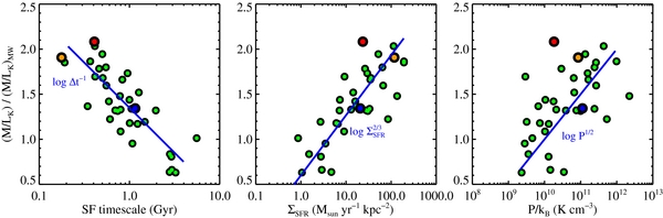
Figure 13. IMF vs. inferred SF timescale (left panel), inferred SFR surface density, ΣSFR (middle panel), and inferred pressure (right panel). All quantities are measured within re/8 except for M31, where quantities are measured within the central 4″ = 15 pc. The quantity plotted on the y-axis is sensitive only to the IMF, as it is the true mass-to-light ratio divided by the mass-to-light ratio assuming a MW IMF. The SF timescale is inferred from the measured [Mg/Fe] abundance. The SFR surface density is estimated from the stellar mass, SF timescale, and present galaxy size, and the pressure is estimated from the mass and present galaxy size. Symbol colors are as in Figure 5. Solid lines are not fits to the points, they are simply intended to guide the eye.
Download figure:
Standard image High-resolution imageWe can go one step further and estimate an average star formation rate (SFR) surface density, ΣSFR, within re/8 based on the stellar mass within this radius,8 M*, and the SF timescale: ΣSF = M*/4πΔt(re/8)2. The result is shown in the middle panel of Figure 13. Galaxies with the most bottom-heavy IMF have inferred SFR surface densities in excess of 100 M☉ yr−1 kpc−2. In the local universe such high SFR surface densities are found only in the most extreme circumnuclear starbursts (Kennicutt 1998). We emphasize that these quantities are based on the present stellar density within re/8. Observations of massive early-type galaxies suggest that their central densities actually decrease with time (Bezanson et al. 2009), which appears to be a consequence of both major and minor mergers (Oser et al. 2012). These inferred SFR surface densities may therefore be lower limits to the true SFR densities.
Another quantity of interest is the pressure of the system, which can be estimated via P∝M2*/r4. We have computed the effective pressure within re/8 for our sample and plotted this against our best-fit IMFs in the right panel of Figure 13. A correlation is apparent, but it is weaker than the other relations shown in this figure. This may be due to the fact that the effective pressure estimated at z = 0 is only weakly correlated with the pressure at the epoch of formation.
In each of these panels we have included simple power-law relations. These were not fits to the data; the power-law indices were chosen by eye to represent the mean trend in the sample.
The data therefore support a scenario wherein the IMF is correlated with the intensity of SF and/or the effective pressure of the system, in the sense that higher SFR densities and higher pressures correspond to more bottom-heavy IMFs.
A number of recent papers have pointed to fragmentation in supersonically turbulent molecular clouds as the key physical process governing the shape of the stellar IMF (Padoan et al. 1997; Padoan & Nordlund 2002; Hennebelle & Chabrier 2008; Hopkins 2012a, 2012b). In this framework, the Mach number within the molecular cloud is a key variable affecting the shape of the IMF. Qualitatively, and for all other variables held fixed, a higher Mach number results in a more bottom-heavy IMF.
As noted above, local circumnuclear starbursts may be analogs to the most massive early-type galaxies in our sample at their formation epoch. The local starbursts have very high SFR densities and have molecular gas that is on average hotter and more supersonically turbulent than the molecular gas in the MW (Downes & Solomon 1998; Bryant & Scoville 1999). The higher Mach numbers in starbursts may be the result of the higher rate of supernovae (SNe) in these systems. Hopkins (2012b) has combined these ideas with an analytic theory for the IMF to demonstrate that such galaxies should have bottom-heavy IMFs. The Mach number is critical to this conclusion: the thermal Jeans mass (MJ∝c3s ρ−1/2, where cs and ρ are the sound speed and density, respectively) in starbursts is frequently larger than in the MW disk, and thus a simple Jeans argument would suggest that the IMF in starbursts should be bottom-light (e.g., Larson 1998; Baugh et al. 2005; Narayanan & Davé 2012). The larger Mach numbers in starbursts overcome the effect of the increasing thermal Jeans mass to result in a lower characteristic mass in the IMF.
The basic idea is that galaxies with higher sustained ΣSFR have a rate per unit volume of SNe which can drive more highly supersonic turbulence, resulting in a higher typical Mach number in molecular clouds that in turn lowers the characteristic mass of the IMF. Note that this picture does not imply that all α-enhanced systems have bottom-heavy IMFs. The ΣSFR must be sustained long enough for the SNe to drive turbulence. In particular, GCs, which are α-enhanced systems, would not be expected to have bottom-heavy IMFs because SF in such systems is approximately instantaneous.
We conclude this section with the caution that isothermality, a key assumption in the models mentioned above, likely does not hold in the regimes of interest. Krumholz (2011) has argued instead that radiative feedback is the key physical process setting the characteristic mass of the IMF, and that the Jeans mass (whether thermal or turbulent) plays no direct role. In Krumholz's model the ISM pressure is the key variable, and there may be some evidence for IMF variation with pressure in Figure 13.
7. SUMMARY
In this paper, we have confronted high-quality absorption line spectra of 38 early-type galaxies and the nuclear bulge of M31 with a new SPS model that incorporates flexible abundance patterns and IMFs. These data and models extend beyond 1 μm, where IMF-sensitive absorption features allow for a strong constraint on the IMF and stellar mass-to-light ratio within individual galaxies. The data sample the inner regions of the galaxies (to re/8) and so conclusions regarding the stellar populations of these galaxies apply strictly to these inner regions. We now summarize our main results.
- 1.Evidence is found for an IMF that varies systematically with galaxy velocity dispersion and α-enhancement. Steeper (more bottom-heavy) IMFs are found in more massive systems. The best-fit mass-to-light ratios do not violate dynamical constraints.
- 2.At the highest velocity dispersions and α-enhancements the IMF becomes steeper than even the canonical Salpeter IMF, with inferred K-band mass-to-light ratios a factor of ≈2 higher than would be expected for a universal, MW IMF.
- 3.Systematic uncertainties in the models translate into ≲ 50% uncertainties in the derived mass-to-light ratios, while the median statistical uncertainty is ≈7%. In particular, there appears to be some tension between the models and data regarding the CaT feature, which is interesting because CaT is strong in giants while the others are strong in dwarfs. We have demonstrated that the tension around the CaT feature is visible for all of the galaxies in our sample and suggests that the relatively poor modeling of the CaT feature does not strongly influence the derived M/L ratios.
- 4.These results are consistent with a scenario wherein the IMF becomes increasingly bottom-heavy as the SF timescale becomes increasingly short, the SFR surface density becomes increasingly high, and/or the ISM pressure becomes increasingly high. These trends are broadly consistent with several recent conjectures for the origin of the IMF, but more detailed models are needed before conclusive statements can be made.
We thank Nelson Caldwell for providing his Hectospec data for the M31 globular clusters, Ricardo Schiavon for assistance with interpreting his models, Michele Cappellari for useful discussions regarding uncertainties in SAURON M/L values, and Jonathan Sick and Stéphane Courteau for providing the nuclear luminosity of M31 from their unpublished data. C.C. thanks Phil Hopkins, Andrey Kravtsov, and Mark Krumholz for informative discussions. We acknowledge use of the Odyssey cluster supported by the FAS Science Division Research Computing Group at Harvard University. Finally, we thank the referee for thoughtful comments that have improved the quality of the manuscript.
The data presented herein were obtained at the W. M. Keck Observatory, which is operated as a scientific partnership among the California Institute of Technology, the University of California and the National Aeronautics and Space Administration. The Observatory was made possible by the generous financial support of the W. M. Keck Foundation. The authors recognize and acknowledge the very significant cultural role and reverence that the summit of Mauna Kea has always had within the indigenous Hawaiian community. We are most fortunate to have the opportunity to conduct observations from this mountain.
APPENDIX
In this Appendix, we provide the fits to all galaxies included in Paper I (excluding NGC 4621 and NGC 524, which are shown in Figures 1 and 2 in the main text; see Figure 14).
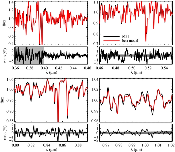
Figure 14.
Fits to all galaxies included in Paper I (excluding NGC 4621 and NGC 524). (A color version and the complete figure set (33 images) are available in the online journal)
Download figure:
Standard image High-resolution imageFootnotes
- 4
The dynamical constraints imply that the mass-to-light ratios are larger than expected for a MW IMF, which can be explained either by a bottom-heavy (dwarf-dominated) IMF or a bottom-light (remnant-dominated) IMF.
- 5
The synthetic spectra are in fact used in an absolute sense to bridge the gap in wavelength coverage between the MILES and IRTF libraries at 0.74 μm–0.8 μm. This wavelength range is not used in the present work.
- 6
K10 quote total metallicity, Z, rather than [Fe/H]. We have converted their results to [Fe/H] via the equation [Fe/H] = Z−0.75[α/Fe]. This relation was derived from tabulated values of [Fe/H], Z, and [α/Fe] kindly provided to us by R. Schiavon.
- 7
- 8
The stellar mass within re/8 is estimated by combining the best-fit M/LK ratios, the total K-band luminosities from Cappellari et al. (2011), and the Sérsic indices from Falcón-Barroso et al. (2011). The latter quantity is used to estimate the fraction of the total light contained within re/8. For M31 the I-band luminosity within our extraction aperture was derived from J. Sick et al. (in preparation).